The Orchestration Engine: Building a Resilient Analysis Pipeline
Event-Driven Architecture & Graph Theory
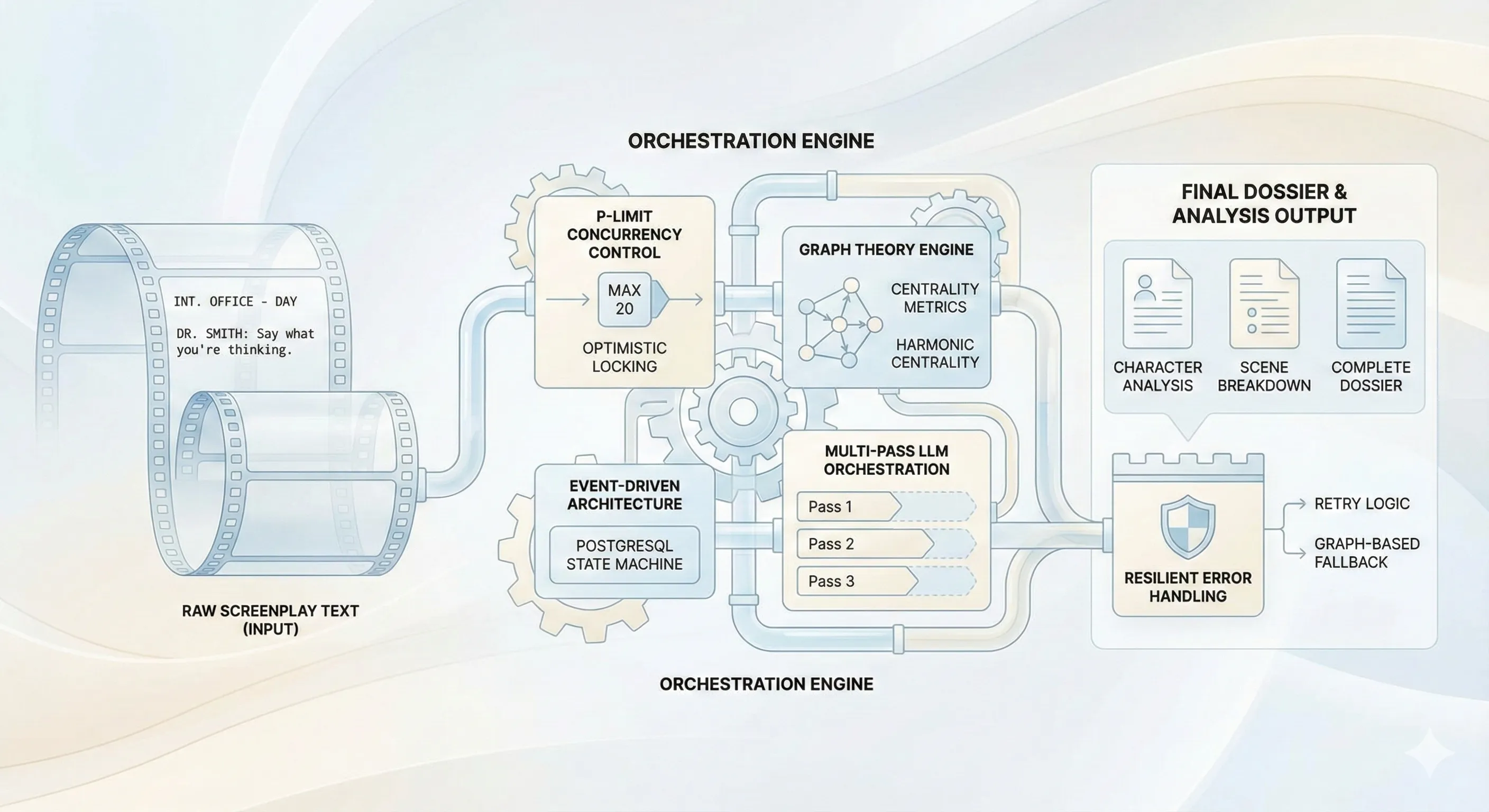
When building scenario-parser, the primary challenge wasn’t just “calling an LLM.” It was orchestration. A typical screenplay analysis involves processing hundreds of entities, thousands of interactions, and maintaining a coherent state across multiple asynchronous stages.
This article dissects the orchestration architecture of Stage 3: Analysis, specifically focusing on concurrency control with p-limit and the implementation of Social Network Analysis (SNA) using graphology.
Note: This article focuses on the analysis pipeline (Stage 3). For the complete system architecture including extraction and our 4-parser competitive strategy, see The Complete Architecture.
The Analysis Pipeline Architecture
The analysis pipeline operates on the best screenplay selected from our 4-parser competitive system. Once we have a high-quality parsed screenplay (Stage 2 complete), we move to Stage 3: Analysis.
The system is designed as a linear, state-aware pipeline with three main artifacts: Synopsis, Character Analysis, and Scene Breakdown. We use an event-driven approach where the completion of one artifact can trigger the processing of dependent artifacts.
Here is the high-level flow of data through the system:
%3b%7d%23mermaid-0 .edgePath .path%7bstroke:%23737373%3bstroke-width:2.0px%3b%7d%23mermaid-0 .flowchart-link%7bstroke:%23737373%3bfill:none%3b%7d%23mermaid-0 .edgeLabel%7bbackground-color:white%3btext-align:center%3b%7d%23mermaid-0 .edgeLabel p%7bbackground-color:white%3b%7d%23mermaid-0 .edgeLabel rect%7bopacity:0.5%3bbackground-color:white%3bfill:white%3b%7d%23mermaid-0 .labelBkg%7bbackground-color:rgba(255%2c 255%2c 255%2c 0.5)%3b%7d%23mermaid-0 .cluster rect%7bfill:white%3bstroke:%23d4d4d4%3bstroke-width:1px%3b%7d%23mermaid-0 .cluster text%7bfill:%23737373%3b%7d%23mermaid-0 .cluster span%7bcolor:%23737373%3b%7d%23mermaid-0 div.mermaidTooltip%7bposition:absolute%3btext-align:center%3bmax-width:200px%3bpadding:2px%3bfont-family:arial%2csans-serif%3bfont-size:12px%3bbackground:%2310b981%3bborder:1px solid hsl(160.1183431953%2c 44.07960199%25%2c 29.4117647059%25)%3bborder-radius:2px%3bpointer-events:none%3bz-index:100%3b%7d%23mermaid-0 .flowchartTitleText%7btext-anchor:middle%3bfont-size:18px%3bfill:%23171717%3b%7d%23mermaid-0 rect.text%7bfill:none%3bstroke-width:0%3b%7d%23mermaid-0 .icon-shape%2c%23mermaid-0 .image-shape%7bbackground-color:white%3btext-align:center%3b%7d%23mermaid-0 .icon-shape p%2c%23mermaid-0 .image-shape p%7bbackground-color:white%3bpadding:2px%3b%7d%23mermaid-0 .icon-shape rect%2c%23mermaid-0 .image-shape rect%7bopacity:0.5%3bbackground-color:white%3bfill:white%3b%7d%23mermaid-0 .label-icon%7bdisplay:inline-block%3bheight:1em%3boverflow:visible%3bvertical-align:-0.125em%3b%7d%23mermaid-0 .node .label-icon path%7bfill:currentColor%3bstroke:revert%3bstroke-width:revert%3b%7d%23mermaid-0 :root%7b--mermaid-font-family:arial%2csans-serif%3b%7d%3c/style%3e%3cg%3e%3cmarker id='mermaid-0_flowchart-v2-pointEnd' class='marker flowchart-v2' viewBox='0 0 10 10' refX='5' refY='5' markerUnits='userSpaceOnUse' markerWidth='8' markerHeight='8' orient='auto'%3e%3cpath d='M 0 0 L 10 5 L 0 10 z' class='arrowMarkerPath' style='stroke-width: 1%3b stroke-dasharray: 1%2c 0%3b'/%3e%3c/marker%3e%3cmarker id='mermaid-0_flowchart-v2-pointStart' class='marker flowchart-v2' viewBox='0 0 10 10' refX='4.5' refY='5' markerUnits='userSpaceOnUse' markerWidth='8' markerHeight='8' orient='auto'%3e%3cpath d='M 0 5 L 10 10 L 10 0 z' class='arrowMarkerPath' style='stroke-width: 1%3b stroke-dasharray: 1%2c 0%3b'/%3e%3c/marker%3e%3cmarker id='mermaid-0_flowchart-v2-circleEnd' class='marker flowchart-v2' viewBox='0 0 10 10' refX='11' refY='5' markerUnits='userSpaceOnUse' markerWidth='11' markerHeight='11' orient='auto'%3e%3ccircle cx='5' cy='5' r='5' class='arrowMarkerPath' style='stroke-width: 1%3b stroke-dasharray: 1%2c 0%3b'/%3e%3c/marker%3e%3cmarker id='mermaid-0_flowchart-v2-circleStart' class='marker flowchart-v2' viewBox='0 0 10 10' refX='-1' refY='5' markerUnits='userSpaceOnUse' markerWidth='11' markerHeight='11' orient='auto'%3e%3ccircle cx='5' cy='5' r='5' class='arrowMarkerPath' style='stroke-width: 1%3b stroke-dasharray: 1%2c 0%3b'/%3e%3c/marker%3e%3cmarker id='mermaid-0_flowchart-v2-crossEnd' class='marker cross flowchart-v2' viewBox='0 0 11 11' refX='12' refY='5.2' markerUnits='userSpaceOnUse' markerWidth='11' markerHeight='11' orient='auto'%3e%3cpath d='M 1%2c1 l 9%2c9 M 10%2c1 l -9%2c9' class='arrowMarkerPath' style='stroke-width: 2%3b stroke-dasharray: 1%2c 0%3b'/%3e%3c/marker%3e%3cmarker id='mermaid-0_flowchart-v2-crossStart' class='marker cross flowchart-v2' viewBox='0 0 11 11' refX='-1' refY='5.2' markerUnits='userSpaceOnUse' markerWidth='11' markerHeight='11' orient='auto'%3e%3cpath d='M 1%2c1 l 9%2c9 M 10%2c1 l -9%2c9' class='arrowMarkerPath' style='stroke-width: 2%3b stroke-dasharray: 1%2c 0%3b'/%3e%3c/marker%3e%3cg class='root'%3e%3cg class='clusters'%3e%3cg class='cluster' id='subGraph3' data-look='classic'%3e%3crect style='' x='26.625' y='1335.15625' width='312.75' height='570'/%3e%3cg class='cluster-label' transform='translate(130.078125%2c 1335.15625)'%3e%3cforeignObject width='105.84375' height='24'%3e%3cdiv xmlns='http://www.w3.org/1999/xhtml' style='display: table-cell%3b white-space: nowrap%3b line-height: 1.5%3b max-width: 200px%3b text-align: center%3b'%3e%3cspan class='nodeLabel'%3e%3cp%3eAnalysis Stage%3c/p%3e%3c/span%3e%3c/div%3e%3c/foreignObject%3e%3c/g%3e%3c/g%3e%3cg class='cluster' id='subGraph2' data-look='classic'%3e%3crect style='' x='8' y='805.15625' width='350' height='480'/%3e%3cg class='cluster-label' transform='translate(132.7421875%2c 805.15625)'%3e%3cforeignObject width='100.515625' height='24'%3e%3cdiv xmlns='http://www.w3.org/1999/xhtml' style='display: table-cell%3b white-space: nowrap%3b line-height: 1.5%3b max-width: 200px%3b text-align: center%3b'%3e%3cspan class='nodeLabel'%3e%3cp%3eParsing Stage%3c/p%3e%3c/span%3e%3c/div%3e%3c/foreignObject%3e%3c/g%3e%3c/g%3e%3cg class='cluster' id='subGraph1' data-look='classic'%3e%3crect style='' x='52.203125' y='286' width='468.296875' height='469.15625'/%3e%3cg class='cluster-label' transform='translate(227.6484375%2c 286)'%3e%3cforeignObject width='117.40625' height='24'%3e%3cdiv xmlns='http://www.w3.org/1999/xhtml' style='display: table-cell%3b white-space: nowrap%3b line-height: 1.5%3b max-width: 200px%3b text-align: center%3b'%3e%3cspan class='nodeLabel'%3e%3cp%3eExtraction Stage%3c/p%3e%3c/span%3e%3c/div%3e%3c/foreignObject%3e%3c/g%3e%3c/g%3e%3cg class='cluster' id='subGraph0' data-look='classic'%3e%3crect style='' x='173.3671875' y='8' width='237.15625' height='228'/%3e%3cg class='cluster-label' transform='translate(251.9140625%2c 8)'%3e%3cforeignObject width='80.0625' height='24'%3e%3cdiv xmlns='http://www.w3.org/1999/xhtml' style='display: table-cell%3b white-space: nowrap%3b line-height: 1.5%3b max-width: 200px%3b text-align: center%3b'%3e%3cspan class='nodeLabel'%3e%3cp%3eInput Layer%3c/p%3e%3c/span%3e%3c/div%3e%3c/foreignObject%3e%3c/g%3e%3c/g%3e%3c/g%3e%3cg class='edgePaths'%3e%3cpath d='M291.945%2c97L291.945%2c101.167C291.945%2c105.333%2c291.945%2c113.667%2c291.945%2c121.333C291.945%2c129%2c291.945%2c136%2c291.945%2c139.5L291.945%2c143' id='L_A_B_0' class='edge-thickness-normal edge-pattern-solid edge-thickness-normal edge-pattern-solid flowchart-link' style='%3b' data-edge='true' data-et='edge' data-id='L_A_B_0' data-points='W3sieCI6MjkxLjk0NTMxMjUsInkiOjk3fSx7IngiOjI5MS45NDUzMTI1LCJ5IjoxMjJ9LHsieCI6MjkxLjk0NTMxMjUsInkiOjE0N31d' marker-end='url(%23mermaid-0_flowchart-v2-pointEnd)'/%3e%3cpath d='M291.945%2c211L291.945%2c215.167C291.945%2c219.333%2c291.945%2c227.667%2c291.945%2c236C291.945%2c244.333%2c291.945%2c252.667%2c291.945%2c261C291.945%2c269.333%2c291.945%2c277.667%2c291.945%2c285.333C291.945%2c293%2c291.945%2c300%2c291.945%2c303.5L291.945%2c307' id='L_B_C_0' class='edge-thickness-normal edge-pattern-solid edge-thickness-normal edge-pattern-solid flowchart-link' style='%3b' data-edge='true' data-et='edge' data-id='L_B_C_0' data-points='W3sieCI6MjkxLjk0NTMxMjUsInkiOjIxMX0seyJ4IjoyOTEuOTQ1MzEyNSwieSI6MjM2fSx7IngiOjI5MS45NDUzMTI1LCJ5IjoyNjF9LHsieCI6MjkxLjk0NTMxMjUsInkiOjI4Nn0seyJ4IjoyOTEuOTQ1MzEyNSwieSI6MzExfV0=' marker-end='url(%23mermaid-0_flowchart-v2-pointEnd)'/%3e%3cpath d='M291.945%2c375L291.945%2c379.167C291.945%2c383.333%2c291.945%2c391.667%2c291.945%2c399.333C291.945%2c407%2c291.945%2c414%2c291.945%2c417.5L291.945%2c421' id='L_C_D_0' class='edge-thickness-normal edge-pattern-solid edge-thickness-normal edge-pattern-solid flowchart-link' style='%3b' data-edge='true' data-et='edge' data-id='L_C_D_0' data-points='W3sieCI6MjkxLjk0NTMxMjUsInkiOjM3NX0seyJ4IjoyOTEuOTQ1MzEyNSwieSI6NDAwfSx7IngiOjI5MS45NDUzMTI1LCJ5Ijo0MjV9XQ==' marker-end='url(%23mermaid-0_flowchart-v2-pointEnd)'/%3e%3cpath d='M252.274%2c552.485L240.729%2c565.264C229.183%2c578.042%2c206.091%2c603.599%2c194.546%2c621.878C183%2c640.156%2c183%2c651.156%2c183%2c656.656L183%2c662.156' id='L_D_E_0' class='edge-thickness-normal edge-pattern-solid edge-thickness-normal edge-pattern-solid flowchart-link' style='%3b' data-edge='true' data-et='edge' data-id='L_D_E_0' data-points='W3sieCI6MjUyLjI3NDIyMjQ5OTQ4OTQ0LCJ5Ijo1NTIuNDg1MTU5OTk5NDg5NH0seyJ4IjoxODMsInkiOjYyOS4xNTYyNX0seyJ4IjoxODMsInkiOjY2Ni4xNTYyNX1d' marker-end='url(%23mermaid-0_flowchart-v2-pointEnd)'/%3e%3cpath d='M331.616%2c552.485L343.162%2c565.264C354.708%2c578.042%2c377.799%2c603.599%2c389.345%2c621.878C400.891%2c640.156%2c400.891%2c651.156%2c400.891%2c656.656L400.891%2c662.156' id='L_D_F_0' class='edge-thickness-normal edge-pattern-solid edge-thickness-normal edge-pattern-solid flowchart-link' style='%3b' data-edge='true' data-et='edge' data-id='L_D_F_0' data-points='W3sieCI6MzMxLjYxNjQwMjUwMDUxMDU2LCJ5Ijo1NTIuNDg1MTU5OTk5NDg5NH0seyJ4Ijo0MDAuODkwNjI1LCJ5Ijo2MjkuMTU2MjV9LHsieCI6NDAwLjg5MDYyNSwieSI6NjY2LjE1NjI1fV0=' marker-end='url(%23mermaid-0_flowchart-v2-pointEnd)'/%3e%3cpath d='M183%2c730.156L183%2c734.323C183%2c738.49%2c183%2c746.823%2c183%2c755.156C183%2c763.49%2c183%2c771.823%2c183%2c780.156C183%2c788.49%2c183%2c796.823%2c183%2c804.49C183%2c812.156%2c183%2c819.156%2c183%2c822.656L183%2c826.156' id='L_E_G_0' class='edge-thickness-normal edge-pattern-solid edge-thickness-normal edge-pattern-solid flowchart-link' style='%3b' data-edge='true' data-et='edge' data-id='L_E_G_0' data-points='W3sieCI6MTgzLCJ5Ijo3MzAuMTU2MjV9LHsieCI6MTgzLCJ5Ijo3NTUuMTU2MjV9LHsieCI6MTgzLCJ5Ijo3ODAuMTU2MjV9LHsieCI6MTgzLCJ5Ijo4MDUuMTU2MjV9LHsieCI6MTgzLCJ5Ijo4MzAuMTU2MjV9XQ==' marker-end='url(%23mermaid-0_flowchart-v2-pointEnd)'/%3e%3cpath d='M183%2c894.156L183%2c898.323C183%2c902.49%2c183%2c910.823%2c183%2c918.49C183%2c926.156%2c183%2c933.156%2c183%2c936.656L183%2c940.156' id='L_G_H_0' class='edge-thickness-normal edge-pattern-solid edge-thickness-normal edge-pattern-solid flowchart-link' style='%3b' data-edge='true' data-et='edge' data-id='L_G_H_0' data-points='W3sieCI6MTgzLCJ5Ijo4OTQuMTU2MjV9LHsieCI6MTgzLCJ5Ijo5MTkuMTU2MjV9LHsieCI6MTgzLCJ5Ijo5NDQuMTU2MjV9XQ==' marker-end='url(%23mermaid-0_flowchart-v2-pointEnd)'/%3e%3cpath d='M183%2c1008.156L183%2c1012.323C183%2c1016.49%2c183%2c1024.823%2c183%2c1032.49C183%2c1040.156%2c183%2c1047.156%2c183%2c1050.656L183%2c1054.156' id='L_H_I_0' class='edge-thickness-normal edge-pattern-solid edge-thickness-normal edge-pattern-solid flowchart-link' style='%3b' data-edge='true' data-et='edge' data-id='L_H_I_0' data-points='W3sieCI6MTgzLCJ5IjoxMDA4LjE1NjI1fSx7IngiOjE4MywieSI6MTAzMy4xNTYyNX0seyJ4IjoxODMsInkiOjEwNTguMTU2MjV9XQ==' marker-end='url(%23mermaid-0_flowchart-v2-pointEnd)'/%3e%3cpath d='M183%2c1122.156L183%2c1126.323C183%2c1130.49%2c183%2c1138.823%2c183%2c1146.49C183%2c1154.156%2c183%2c1161.156%2c183%2c1164.656L183%2c1168.156' id='L_I_J_0' class='edge-thickness-normal edge-pattern-solid edge-thickness-normal edge-pattern-solid flowchart-link' style='%3b' data-edge='true' data-et='edge' data-id='L_I_J_0' data-points='W3sieCI6MTgzLCJ5IjoxMTIyLjE1NjI1fSx7IngiOjE4MywieSI6MTE0Ny4xNTYyNX0seyJ4IjoxODMsInkiOjExNzIuMTU2MjV9XQ==' marker-end='url(%23mermaid-0_flowchart-v2-pointEnd)'/%3e%3cpath d='M183%2c1260.156L183%2c1264.323C183%2c1268.49%2c183%2c1276.823%2c183%2c1285.156C183%2c1293.49%2c183%2c1301.823%2c183%2c1310.156C183%2c1318.49%2c183%2c1326.823%2c183%2c1334.49C183%2c1342.156%2c183%2c1349.156%2c183%2c1352.656L183%2c1356.156' id='L_J_K_0' class='edge-thickness-normal edge-pattern-solid edge-thickness-normal edge-pattern-solid flowchart-link' style='%3b' data-edge='true' data-et='edge' data-id='L_J_K_0' data-points='W3sieCI6MTgzLCJ5IjoxMjYwLjE1NjI1fSx7IngiOjE4MywieSI6MTI4NS4xNTYyNX0seyJ4IjoxODMsInkiOjEzMTAuMTU2MjV9LHsieCI6MTgzLCJ5IjoxMzM1LjE1NjI1fSx7IngiOjE4MywieSI6MTM2MC4xNTYyNX1d' marker-end='url(%23mermaid-0_flowchart-v2-pointEnd)'/%3e%3cpath d='M183%2c1424.156L183%2c1428.323C183%2c1432.49%2c183%2c1440.823%2c183%2c1448.49C183%2c1456.156%2c183%2c1463.156%2c183%2c1466.656L183%2c1470.156' id='L_K_L_0' class='edge-thickness-normal edge-pattern-solid edge-thickness-normal edge-pattern-solid flowchart-link' style='%3b' data-edge='true' data-et='edge' data-id='L_K_L_0' data-points='W3sieCI6MTgzLCJ5IjoxNDI0LjE1NjI1fSx7IngiOjE4MywieSI6MTQ0OS4xNTYyNX0seyJ4IjoxODMsInkiOjE0NzQuMTU2MjV9XQ==' marker-end='url(%23mermaid-0_flowchart-v2-pointEnd)'/%3e%3cpath d='M183%2c1538.156L183%2c1542.323C183%2c1546.49%2c183%2c1554.823%2c183%2c1562.49C183%2c1570.156%2c183%2c1577.156%2c183%2c1580.656L183%2c1584.156' id='L_L_M_0' class='edge-thickness-normal edge-pattern-solid edge-thickness-normal edge-pattern-solid flowchart-link' style='%3b' data-edge='true' data-et='edge' data-id='L_L_M_0' data-points='W3sieCI6MTgzLCJ5IjoxNTM4LjE1NjI1fSx7IngiOjE4MywieSI6MTU2My4xNTYyNX0seyJ4IjoxODMsInkiOjE1ODguMTU2MjV9XQ==' marker-end='url(%23mermaid-0_flowchart-v2-pointEnd)'/%3e%3cpath d='M183%2c1652.156L183%2c1656.323C183%2c1660.49%2c183%2c1668.823%2c183%2c1676.49C183%2c1684.156%2c183%2c1691.156%2c183%2c1694.656L183%2c1698.156' id='L_M_N_0' class='edge-thickness-normal edge-pattern-solid edge-thickness-normal edge-pattern-solid flowchart-link' style='%3b' data-edge='true' data-et='edge' data-id='L_M_N_0' data-points='W3sieCI6MTgzLCJ5IjoxNjUyLjE1NjI1fSx7IngiOjE4MywieSI6MTY3Ny4xNTYyNX0seyJ4IjoxODMsInkiOjE3MDIuMTU2MjV9XQ==' marker-end='url(%23mermaid-0_flowchart-v2-pointEnd)'/%3e%3cpath d='M183%2c1766.156L183%2c1770.323C183%2c1774.49%2c183%2c1782.823%2c183%2c1790.49C183%2c1798.156%2c183%2c1805.156%2c183%2c1808.656L183%2c1812.156' id='L_N_O_0' class='edge-thickness-normal edge-pattern-solid edge-thickness-normal edge-pattern-solid flowchart-link' style='%3b' data-edge='true' data-et='edge' data-id='L_N_O_0' data-points='W3sieCI6MTgzLCJ5IjoxNzY2LjE1NjI1fSx7IngiOjE4MywieSI6MTc5MS4xNTYyNX0seyJ4IjoxODMsInkiOjE4MTYuMTU2MjV9XQ==' marker-end='url(%23mermaid-0_flowchart-v2-pointEnd)'/%3e%3c/g%3e%3cg class='edgeLabels'%3e%3cg class='edgeLabel'%3e%3cg class='label' data-id='L_A_B_0' transform='translate(0%2c 0)'%3e%3cforeignObject width='0' height='0'%3e%3cdiv xmlns='http://www.w3.org/1999/xhtml' class='labelBkg' style='display: table-cell%3b white-space: nowrap%3b line-height: 1.5%3b max-width: 200px%3b text-align: center%3b'%3e%3cspan class='edgeLabel'%3e%3c/span%3e%3c/div%3e%3c/foreignObject%3e%3c/g%3e%3c/g%3e%3cg class='edgeLabel'%3e%3cg class='label' data-id='L_B_C_0' transform='translate(0%2c 0)'%3e%3cforeignObject width='0' height='0'%3e%3cdiv xmlns='http://www.w3.org/1999/xhtml' class='labelBkg' style='display: table-cell%3b white-space: nowrap%3b line-height: 1.5%3b max-width: 200px%3b text-align: center%3b'%3e%3cspan class='edgeLabel'%3e%3c/span%3e%3c/div%3e%3c/foreignObject%3e%3c/g%3e%3c/g%3e%3cg class='edgeLabel'%3e%3cg class='label' data-id='L_C_D_0' transform='translate(0%2c 0)'%3e%3cforeignObject width='0' height='0'%3e%3cdiv xmlns='http://www.w3.org/1999/xhtml' class='labelBkg' style='display: table-cell%3b white-space: nowrap%3b line-height: 1.5%3b max-width: 200px%3b text-align: center%3b'%3e%3cspan class='edgeLabel'%3e%3c/span%3e%3c/div%3e%3c/foreignObject%3e%3c/g%3e%3c/g%3e%3cg class='edgeLabel' transform='translate(183%2c 629.15625)'%3e%3cg class='label' data-id='L_D_E_0' transform='translate(-36.90625%2c -12)'%3e%3cforeignObject width='73.8125' height='24'%3e%3cdiv xmlns='http://www.w3.org/1999/xhtml' class='labelBkg' style='display: table-cell%3b white-space: nowrap%3b line-height: 1.5%3b max-width: 200px%3b text-align: center%3b'%3e%3cspan class='edgeLabel'%3e%3cp%3eMarkdown%3c/p%3e%3c/span%3e%3c/div%3e%3c/foreignObject%3e%3c/g%3e%3c/g%3e%3cg class='edgeLabel' transform='translate(400.890625%2c 629.15625)'%3e%3cg class='label' data-id='L_D_F_0' transform='translate(-34.5390625%2c -12)'%3e%3cforeignObject width='69.078125' height='24'%3e%3cdiv xmlns='http://www.w3.org/1999/xhtml' class='labelBkg' style='display: table-cell%3b white-space: nowrap%3b line-height: 1.5%3b max-width: 200px%3b text-align: center%3b'%3e%3cspan class='edgeLabel'%3e%3cp%3ePlain Text%3c/p%3e%3c/span%3e%3c/div%3e%3c/foreignObject%3e%3c/g%3e%3c/g%3e%3cg class='edgeLabel'%3e%3cg class='label' data-id='L_E_G_0' transform='translate(0%2c 0)'%3e%3cforeignObject width='0' height='0'%3e%3cdiv xmlns='http://www.w3.org/1999/xhtml' class='labelBkg' style='display: table-cell%3b white-space: nowrap%3b line-height: 1.5%3b max-width: 200px%3b text-align: center%3b'%3e%3cspan class='edgeLabel'%3e%3c/span%3e%3c/div%3e%3c/foreignObject%3e%3c/g%3e%3c/g%3e%3cg class='edgeLabel'%3e%3cg class='label' data-id='L_G_H_0' transform='translate(0%2c 0)'%3e%3cforeignObject width='0' height='0'%3e%3cdiv xmlns='http://www.w3.org/1999/xhtml' class='labelBkg' style='display: table-cell%3b white-space: nowrap%3b line-height: 1.5%3b max-width: 200px%3b text-align: center%3b'%3e%3cspan class='edgeLabel'%3e%3c/span%3e%3c/div%3e%3c/foreignObject%3e%3c/g%3e%3c/g%3e%3cg class='edgeLabel'%3e%3cg class='label' data-id='L_H_I_0' transform='translate(0%2c 0)'%3e%3cforeignObject width='0' height='0'%3e%3cdiv xmlns='http://www.w3.org/1999/xhtml' class='labelBkg' style='display: table-cell%3b white-space: nowrap%3b line-height: 1.5%3b max-width: 200px%3b text-align: center%3b'%3e%3cspan class='edgeLabel'%3e%3c/span%3e%3c/div%3e%3c/foreignObject%3e%3c/g%3e%3c/g%3e%3cg class='edgeLabel'%3e%3cg class='label' data-id='L_I_J_0' transform='translate(0%2c 0)'%3e%3cforeignObject width='0' height='0'%3e%3cdiv xmlns='http://www.w3.org/1999/xhtml' class='labelBkg' style='display: table-cell%3b white-space: nowrap%3b line-height: 1.5%3b max-width: 200px%3b text-align: center%3b'%3e%3cspan class='edgeLabel'%3e%3c/span%3e%3c/div%3e%3c/foreignObject%3e%3c/g%3e%3c/g%3e%3cg class='edgeLabel'%3e%3cg class='label' data-id='L_J_K_0' transform='translate(0%2c 0)'%3e%3cforeignObject width='0' height='0'%3e%3cdiv xmlns='http://www.w3.org/1999/xhtml' class='labelBkg' style='display: table-cell%3b white-space: nowrap%3b line-height: 1.5%3b max-width: 200px%3b text-align: center%3b'%3e%3cspan class='edgeLabel'%3e%3c/span%3e%3c/div%3e%3c/foreignObject%3e%3c/g%3e%3c/g%3e%3cg class='edgeLabel'%3e%3cg class='label' data-id='L_K_L_0' transform='translate(0%2c 0)'%3e%3cforeignObject width='0' height='0'%3e%3cdiv xmlns='http://www.w3.org/1999/xhtml' class='labelBkg' style='display: table-cell%3b white-space: nowrap%3b line-height: 1.5%3b max-width: 200px%3b text-align: center%3b'%3e%3cspan class='edgeLabel'%3e%3c/span%3e%3c/div%3e%3c/foreignObject%3e%3c/g%3e%3c/g%3e%3cg class='edgeLabel'%3e%3cg class='label' data-id='L_L_M_0' transform='translate(0%2c 0)'%3e%3cforeignObject width='0' height='0'%3e%3cdiv xmlns='http://www.w3.org/1999/xhtml' class='labelBkg' style='display: table-cell%3b white-space: nowrap%3b line-height: 1.5%3b max-width: 200px%3b text-align: center%3b'%3e%3cspan class='edgeLabel'%3e%3c/span%3e%3c/div%3e%3c/foreignObject%3e%3c/g%3e%3c/g%3e%3cg class='edgeLabel'%3e%3cg class='label' data-id='L_M_N_0' transform='translate(0%2c 0)'%3e%3cforeignObject width='0' height='0'%3e%3cdiv xmlns='http://www.w3.org/1999/xhtml' class='labelBkg' style='display: table-cell%3b white-space: nowrap%3b line-height: 1.5%3b max-width: 200px%3b text-align: center%3b'%3e%3cspan class='edgeLabel'%3e%3c/span%3e%3c/div%3e%3c/foreignObject%3e%3c/g%3e%3c/g%3e%3cg class='edgeLabel'%3e%3cg class='label' data-id='L_N_O_0' transform='translate(0%2c 0)'%3e%3cforeignObject width='0' height='0'%3e%3cdiv xmlns='http://www.w3.org/1999/xhtml' class='labelBkg' style='display: table-cell%3b white-space: nowrap%3b line-height: 1.5%3b max-width: 200px%3b text-align: center%3b'%3e%3cspan class='edgeLabel'%3e%3c/span%3e%3c/div%3e%3c/foreignObject%3e%3c/g%3e%3c/g%3e%3c/g%3e%3cg class='nodes'%3e%3cg class='node default' id='flowchart-A-0' transform='translate(291.9453125%2c 65)'%3e%3crect class='basic label-container' style='fill:%23f9f !important%3bstroke:%23333 !important%3bstroke-width:2px !important' x='-83.578125' y='-32' width='167.15625' height='64'/%3e%3cg class='label' style='' transform='translate(-43.578125%2c -12)'%3e%3crect/%3e%3cforeignObject width='87.15625' height='24'%3e%3cdiv xmlns='http://www.w3.org/1999/xhtml' style='display: table-cell%3b white-space: nowrap%3b line-height: 1.5%3b max-width: 200px%3b text-align: center%3b'%3e%3cspan class='nodeLabel'%3e%3cp%3eUpload PDF%3c/p%3e%3c/span%3e%3c/div%3e%3c/foreignObject%3e%3c/g%3e%3c/g%3e%3cg class='node default' id='flowchart-B-1' transform='translate(291.9453125%2c 179)'%3e%3crect class='basic label-container' style='' x='-79.140625' y='-32' width='158.28125' height='64'/%3e%3cg class='label' style='' transform='translate(-39.140625%2c -12)'%3e%3crect/%3e%3cforeignObject width='78.28125' height='24'%3e%3cdiv xmlns='http://www.w3.org/1999/xhtml' style='display: table-cell%3b white-space: nowrap%3b line-height: 1.5%3b max-width: 200px%3b text-align: center%3b'%3e%3cspan class='nodeLabel'%3e%3cp%3eQueue Job%3c/p%3e%3c/span%3e%3c/div%3e%3c/foreignObject%3e%3c/g%3e%3c/g%3e%3cg class='node default' id='flowchart-C-3' transform='translate(291.9453125%2c 343)'%3e%3crect class='basic label-container' style='' x='-96.4609375' y='-32' width='192.921875' height='64'/%3e%3cg class='label' style='' transform='translate(-56.4609375%2c -12)'%3e%3crect/%3e%3cforeignObject width='112.921875' height='24'%3e%3cdiv xmlns='http://www.w3.org/1999/xhtml' style='display: table-cell%3b white-space: nowrap%3b line-height: 1.5%3b max-width: 200px%3b text-align: center%3b'%3e%3cspan class='nodeLabel'%3e%3cp%3ePyMuPDF4LLM%3c/p%3e%3c/span%3e%3c/div%3e%3c/foreignObject%3e%3c/g%3e%3c/g%3e%3cg class='node default' id='flowchart-D-5' transform='translate(291.9453125%2c 508.578125)'%3e%3cpolygon points='83.578125%2c0 167.15625%2c-83.578125 83.578125%2c-167.15625 0%2c-83.578125' class='label-container' transform='translate(-83.078125%2c 83.578125)'/%3e%3cg class='label' style='' transform='translate(-51.578125%2c -12)'%3e%3crect/%3e%3cforeignObject width='103.15625' height='24'%3e%3cdiv xmlns='http://www.w3.org/1999/xhtml' style='display: table-cell%3b white-space: nowrap%3b line-height: 1.5%3b max-width: 200px%3b text-align: center%3b'%3e%3cspan class='nodeLabel'%3e%3cp%3eOutput Format%3c/p%3e%3c/span%3e%3c/div%3e%3c/foreignObject%3e%3c/g%3e%3c/g%3e%3cg class='node default' id='flowchart-E-7' transform='translate(183%2c 698.15625)'%3e%3crect class='basic label-container' style='' x='-95.1328125' y='-32' width='190.265625' height='64'/%3e%3cg class='label' style='' transform='translate(-55.1328125%2c -12)'%3e%3crect/%3e%3cforeignObject width='110.265625' height='24'%3e%3cdiv xmlns='http://www.w3.org/1999/xhtml' style='display: table-cell%3b white-space: nowrap%3b line-height: 1.5%3b max-width: 200px%3b text-align: center%3b'%3e%3cspan class='nodeLabel'%3e%3cp%3eRaw Markdown%3c/p%3e%3c/span%3e%3c/div%3e%3c/foreignObject%3e%3c/g%3e%3c/g%3e%3cg class='node default' id='flowchart-F-9' transform='translate(400.890625%2c 698.15625)'%3e%3crect class='basic label-container' style='' x='-72.7578125' y='-32' width='145.515625' height='64'/%3e%3cg class='label' style='' transform='translate(-32.7578125%2c -12)'%3e%3crect/%3e%3cforeignObject width='65.515625' height='24'%3e%3cdiv xmlns='http://www.w3.org/1999/xhtml' style='display: table-cell%3b white-space: nowrap%3b line-height: 1.5%3b max-width: 200px%3b text-align: center%3b'%3e%3cspan class='nodeLabel'%3e%3cp%3eRaw Text%3c/p%3e%3c/span%3e%3c/div%3e%3c/foreignObject%3e%3c/g%3e%3c/g%3e%3cg class='node default' id='flowchart-G-11' transform='translate(183%2c 862.15625)'%3e%3crect class='basic label-container' style='' x='-98.2421875' y='-32' width='196.484375' height='64'/%3e%3cg class='label' style='' transform='translate(-58.2421875%2c -12)'%3e%3crect/%3e%3cforeignObject width='116.484375' height='24'%3e%3cdiv xmlns='http://www.w3.org/1999/xhtml' style='display: table-cell%3b white-space: nowrap%3b line-height: 1.5%3b max-width: 200px%3b text-align: center%3b'%3e%3cspan class='nodeLabel'%3e%3cp%3eRegex Classifier%3c/p%3e%3c/span%3e%3c/div%3e%3c/foreignObject%3e%3c/g%3e%3c/g%3e%3cg class='node default' id='flowchart-H-13' transform='translate(183%2c 976.15625)'%3e%3crect class='basic label-container' style='' x='-97.359375' y='-32' width='194.71875' height='64'/%3e%3cg class='label' style='' transform='translate(-57.359375%2c -12)'%3e%3crect/%3e%3cforeignObject width='114.71875' height='24'%3e%3cdiv xmlns='http://www.w3.org/1999/xhtml' style='display: table-cell%3b white-space: nowrap%3b line-height: 1.5%3b max-width: 200px%3b text-align: center%3b'%3e%3cspan class='nodeLabel'%3e%3cp%3eElement Stream%3c/p%3e%3c/span%3e%3c/div%3e%3c/foreignObject%3e%3c/g%3e%3c/g%3e%3cg class='node default' id='flowchart-I-15' transform='translate(183%2c 1090.15625)'%3e%3crect class='basic label-container' style='' x='-91.140625' y='-32' width='182.28125' height='64'/%3e%3cg class='label' style='' transform='translate(-51.140625%2c -12)'%3e%3crect/%3e%3cforeignObject width='102.28125' height='24'%3e%3cdiv xmlns='http://www.w3.org/1999/xhtml' style='display: table-cell%3b white-space: nowrap%3b line-height: 1.5%3b max-width: 200px%3b text-align: center%3b'%3e%3cspan class='nodeLabel'%3e%3cp%3eState Machine%3c/p%3e%3c/span%3e%3c/div%3e%3c/foreignObject%3e%3c/g%3e%3c/g%3e%3cg class='node default' id='flowchart-J-17' transform='translate(183%2c 1216.15625)'%3e%3crect class='basic label-container' style='' x='-140' y='-44' width='280' height='88'/%3e%3cg class='label' style='' transform='translate(-100%2c -24)'%3e%3crect/%3e%3cforeignObject width='200' height='48'%3e%3cdiv xmlns='http://www.w3.org/1999/xhtml' style='display: table%3b white-space: break-spaces%3b line-height: 1.5%3b max-width: 200px%3b text-align: center%3b width: 200px%3b'%3e%3cspan class='nodeLabel'%3e%3cp%3eStructured Screenplay JSON%3c/p%3e%3c/span%3e%3c/div%3e%3c/foreignObject%3e%3c/g%3e%3c/g%3e%3cg class='node default' id='flowchart-K-19' transform='translate(183%2c 1392.15625)'%3e%3crect class='basic label-container' style='' x='-116.0234375' y='-32' width='232.046875' height='64'/%3e%3cg class='label' style='' transform='translate(-76.0234375%2c -12)'%3e%3crect/%3e%3cforeignObject width='152.046875' height='24'%3e%3cdiv xmlns='http://www.w3.org/1999/xhtml' style='display: table-cell%3b white-space: nowrap%3b line-height: 1.5%3b max-width: 200px%3b text-align: center%3b'%3e%3cspan class='nodeLabel'%3e%3cp%3eCharacter Normalizer%3c/p%3e%3c/span%3e%3c/div%3e%3c/foreignObject%3e%3c/g%3e%3c/g%3e%3cg class='node default' id='flowchart-L-21' transform='translate(183%2c 1506.15625)'%3e%3crect class='basic label-container' style='' x='-89.359375' y='-32' width='178.71875' height='64'/%3e%3cg class='label' style='' transform='translate(-49.359375%2c -12)'%3e%3crect/%3e%3cforeignObject width='98.71875' height='24'%3e%3cdiv xmlns='http://www.w3.org/1999/xhtml' style='display: table-cell%3b white-space: nowrap%3b line-height: 1.5%3b max-width: 200px%3b text-align: center%3b'%3e%3cspan class='nodeLabel'%3e%3cp%3eGraph Builder%3c/p%3e%3c/span%3e%3c/div%3e%3c/foreignObject%3e%3c/g%3e%3c/g%3e%3cg class='node default' id='flowchart-M-23' transform='translate(183%2c 1620.15625)'%3e%3crect class='basic label-container' style='' x='-121.375' y='-32' width='242.75' height='64'/%3e%3cg class='label' style='' transform='translate(-81.375%2c -12)'%3e%3crect/%3e%3cforeignObject width='162.75' height='24'%3e%3cdiv xmlns='http://www.w3.org/1999/xhtml' style='display: table-cell%3b white-space: nowrap%3b line-height: 1.5%3b max-width: 200px%3b text-align: center%3b'%3e%3cspan class='nodeLabel'%3e%3cp%3eCentrality Computation%3c/p%3e%3c/span%3e%3c/div%3e%3c/foreignObject%3e%3c/g%3e%3c/g%3e%3cg class='node default' id='flowchart-N-25' transform='translate(183%2c 1734.15625)'%3e%3crect class='basic label-container' style='' x='-112.4765625' y='-32' width='224.953125' height='64'/%3e%3cg class='label' style='' transform='translate(-72.4765625%2c -12)'%3e%3crect/%3e%3cforeignObject width='144.953125' height='24'%3e%3cdiv xmlns='http://www.w3.org/1999/xhtml' style='display: table-cell%3b white-space: nowrap%3b line-height: 1.5%3b max-width: 200px%3b text-align: center%3b'%3e%3cspan class='nodeLabel'%3e%3cp%3eLLM Synthesis Pass%3c/p%3e%3c/span%3e%3c/div%3e%3c/foreignObject%3e%3c/g%3e%3c/g%3e%3cg class='node default' id='flowchart-O-27' transform='translate(183%2c 1848.15625)'%3e%3crect class='basic label-container' style='fill:%239f9 !important%3bstroke:%23333 !important%3bstroke-width:2px !important' x='-86.6796875' y='-32' width='173.359375' height='64'/%3e%3cg class='label' style='' transform='translate(-46.6796875%2c -12)'%3e%3crect/%3e%3cforeignObject width='93.359375' height='24'%3e%3cdiv xmlns='http://www.w3.org/1999/xhtml' style='display: table-cell%3b white-space: nowrap%3b line-height: 1.5%3b max-width: 200px%3b text-align: center%3b'%3e%3cspan class='nodeLabel'%3e%3cp%3eFinal Dossier%3c/p%3e%3c/span%3e%3c/div%3e%3c/foreignObject%3e%3c/g%3e%3c/g%3e%3c/g%3e%3c/g%3e%3c/g%3e%3c/svg%3e)
Event-Driven Flow with Artifact State Machine
The pipeline operates on an artifact-based state machine. Each artifact (extraction result, parsed screenplay, character analysis) progresses through distinct states tracked in PostgreSQL:
%3bfill:%23fff5ad%3b%7d%23mermaid-1 .state-note text%7bfill:%23333%3bstroke:none%3bfont-size:10px%3b%7d%23mermaid-1 .stateLabel .box%7bstroke:none%3bstroke-width:0%3bfill:white%3bopacity:0.5%3b%7d%23mermaid-1 .edgeLabel .label rect%7bfill:white%3bopacity:0.5%3b%7d%23mermaid-1 .edgeLabel%7bbackground-color:white%3btext-align:center%3b%7d%23mermaid-1 .edgeLabel p%7bbackground-color:white%3b%7d%23mermaid-1 .edgeLabel rect%7bopacity:0.5%3bbackground-color:white%3bfill:white%3b%7d%23mermaid-1 .edgeLabel .label text%7bfill:%23171717%3b%7d%23mermaid-1 .label div .edgeLabel%7bcolor:%23171717%3b%7d%23mermaid-1 .stateLabel text%7bfill:%23171717%3bfont-size:10px%3bfont-weight:bold%3b%7d%23mermaid-1 .node circle.state-start%7bfill:%23737373%3bstroke:%23737373%3b%7d%23mermaid-1 .node .fork-join%7bfill:%23737373%3bstroke:%23737373%3b%7d%23mermaid-1 .node circle.state-end%7bfill:%23a3a3a3%3bstroke:transparent%3bstroke-width:1.5%3b%7d%23mermaid-1 .end-state-inner%7bfill:transparent%3bstroke-width:1.5%3b%7d%23mermaid-1 .node rect%7bfill:white%3bstroke:%23a3a3a3%3bstroke-width:1px%3b%7d%23mermaid-1 .node polygon%7bfill:white%3bstroke:%23a3a3a3%3bstroke-width:1px%3b%7d%23mermaid-1 %23statediagram-barbEnd%7bfill:%23737373%3b%7d%23mermaid-1 .statediagram-cluster rect%7bfill:white%3bstroke:%23a3a3a3%3bstroke-width:1px%3b%7d%23mermaid-1 .cluster-label%2c%23mermaid-1 .nodeLabel%7bcolor:%23171717%3b%7d%23mermaid-1 .statediagram-cluster rect.outer%7brx:5px%3bry:5px%3b%7d%23mermaid-1 .statediagram-state .divider%7bstroke:%23a3a3a3%3b%7d%23mermaid-1 .statediagram-state .title-state%7brx:5px%3bry:5px%3b%7d%23mermaid-1 .statediagram-cluster.statediagram-cluster .inner%7bfill:transparent%3b%7d%23mermaid-1 .statediagram-cluster.statediagram-cluster-alt .inner%7bfill:%2310b981%3b%7d%23mermaid-1 .statediagram-cluster .inner%7brx:0%3bry:0%3b%7d%23mermaid-1 .statediagram-state rect.basic%7brx:5px%3bry:5px%3b%7d%23mermaid-1 .statediagram-state rect.divider%7bstroke-dasharray:10%2c10%3bfill:%2310b981%3b%7d%23mermaid-1 .note-edge%7bstroke-dasharray:5%3b%7d%23mermaid-1 .statediagram-note rect%7bfill:%23fff5ad%3bstroke:hsl(52.6829268293%2c 60%25%2c 73.9215686275%25)%3bstroke-width:1px%3brx:0%3bry:0%3b%7d%23mermaid-1 .statediagram-note rect%7bfill:%23fff5ad%3bstroke:hsl(52.6829268293%2c 60%25%2c 73.9215686275%25)%3bstroke-width:1px%3brx:0%3bry:0%3b%7d%23mermaid-1 .statediagram-note text%7bfill:%23333%3b%7d%23mermaid-1 .statediagram-note .nodeLabel%7bcolor:%23333%3b%7d%23mermaid-1 .statediagram .edgeLabel%7bcolor:red%3b%7d%23mermaid-1 %23dependencyStart%2c%23mermaid-1 %23dependencyEnd%7bfill:%23737373%3bstroke:%23737373%3bstroke-width:1%3b%7d%23mermaid-1 .statediagramTitleText%7btext-anchor:middle%3bfont-size:18px%3bfill:%23171717%3b%7d%23mermaid-1 :root%7b--mermaid-font-family:arial%2csans-serif%3b%7d%3c/style%3e%3cg%3e%3cdefs%3e%3cmarker id='mermaid-1_stateDiagram-barbEnd' refX='19' refY='7' markerWidth='20' markerHeight='14' markerUnits='userSpaceOnUse' orient='auto'%3e%3cpath d='M 19%2c7 L9%2c13 L14%2c7 L9%2c1 Z'/%3e%3c/marker%3e%3c/defs%3e%3cg class='root'%3e%3cg class='clusters'%3e%3cg class='note-cluster' id='Processing----parent'%3e%3crect x='8' y='324' width='300.296875' height='138' fill='none'/%3e%3c/g%3e%3cg class='note-cluster' id='Failed----parent'%3e%3crect x='450.5970733165741' y='512' width='280.765625' height='138' fill='none'/%3e%3c/g%3e%3c/g%3e%3cg class='edgePaths'%3e%3cpath d='M499.785%2c22L499.785%2c28.167C499.785%2c34.333%2c499.785%2c46.667%2c499.868%2c59.083C499.952%2c71.5%2c500.118%2c84%2c500.202%2c90.25L500.285%2c96.5' id='edge0' class='edge-thickness-normal edge-pattern-solid transition' style='fill:none%3b%3b%3bfill:none' data-edge='true' data-et='edge' data-id='edge0' data-points='W3sieCI6NDk5Ljc4NTE1NjI1LCJ5IjoyMn0seyJ4Ijo0OTkuNzg1MTU2MjUsInkiOjU5fSx7IngiOjUwMC4yODUxNTYyNSwieSI6OTYuNX1d' marker-end='url(%23mermaid-1_stateDiagram-barbEnd)'/%3e%3cpath d='M464.459%2c135.098L452.047%2c141.415C439.634%2c147.732%2c414.809%2c160.366%2c402.48%2c172.933C390.151%2c185.5%2c390.318%2c198%2c390.401%2c204.25L390.484%2c210.5' id='edge1' class='edge-thickness-normal edge-pattern-solid transition' style='fill:none%3b%3b%3bfill:none' data-edge='true' data-et='edge' data-id='edge1' data-points='W3sieCI6NDY0LjQ1ODkzMzc0MDM1MDIsInkiOjEzNS4wOTgxNzk5MDE4Mzk2NH0seyJ4IjozODkuOTg0Mzc1LCJ5IjoxNzN9LHsieCI6MzkwLjQ4NDM3NSwieSI6MjEwLjV9XQ==' marker-end='url(%23mermaid-1_stateDiagram-barbEnd)'/%3e%3cpath d='M390.484%2c250.5L390.401%2c256.583C390.318%2c262.667%2c390.151%2c274.833%2c390.068%2c287.083C389.984%2c299.333%2c389.984%2c311.667%2c390.068%2c326.083C390.151%2c340.5%2c390.318%2c357%2c390.401%2c365.25L390.484%2c373.5' id='edge2' class='edge-thickness-normal edge-pattern-solid transition' style='fill:none%3b%3b%3bfill:none' data-edge='true' data-et='edge' data-id='edge2' data-points='W3sieCI6MzkwLjQ4NDM3NSwieSI6MjUwLjV9LHsieCI6Mzg5Ljk4NDM3NSwieSI6Mjg3fSx7IngiOjM4OS45ODQzNzUsInkiOjMyNH0seyJ4IjozOTAuNDg0Mzc1LCJ5IjozNzMuNX1d' marker-end='url(%23mermaid-1_stateDiagram-barbEnd)'/%3e%3cpath d='M437.837%2c246.97L457.175%2c253.642C476.512%2c260.313%2c515.188%2c273.657%2c534.525%2c286.495C553.863%2c299.333%2c553.863%2c311.667%2c558.339%2c326.083C562.816%2c340.5%2c571.768%2c357%2c576.245%2c365.25L580.721%2c373.5' id='edge3' class='edge-thickness-normal edge-pattern-solid transition' style='fill:none%3b%3b%3bfill:none' data-edge='true' data-et='edge' data-id='edge3' data-points='W3sieCI6NDM3LjgzNzIxODc1MDY1NjYzLCJ5IjoyNDYuOTcwMjIwMzM4ODYzMTZ9LHsieCI6NTUzLjg2MjY5ODMxNjU3NDEsInkiOjI4N30seyJ4Ijo1NTMuODYyNjk4MzE2NTc0MSwieSI6MzI0fSx7IngiOjU4MC43MjEyODA3NDQxMTAzLCJ5IjozNzMuNX1d' marker-end='url(%23mermaid-1_stateDiagram-barbEnd)'/%3e%3cpath d='M602.238%2c373.5L606.548%2c365.25C610.858%2c357%2c619.478%2c340.5%2c623.787%2c326.083C628.097%2c311.667%2c628.097%2c299.333%2c628.097%2c283.667C628.097%2c268%2c628.097%2c249%2c628.097%2c230C628.097%2c211%2c628.097%2c192%2c612.983%2c175.832C597.869%2c159.664%2c567.641%2c146.329%2c552.527%2c139.661L537.412%2c132.993' id='edge4' class='edge-thickness-normal edge-pattern-solid transition' style='fill:none%3b%3b%3bfill:none' data-edge='true' data-et='edge' data-id='edge4' data-points='W3sieCI6NjAyLjIzODQ5MDg4OTAzNzgsInkiOjM3My41fSx7IngiOjYyOC4wOTcwNzMzMTY1NzQxLCJ5IjozMjR9LHsieCI6NjI4LjA5NzA3MzMxNjU3NDEsInkiOjI4N30seyJ4Ijo2MjguMDk3MDczMzE2NTc0MSwieSI6MjMwfSx7IngiOjYyOC4wOTcwNzMzMTY1NzQxLCJ5IjoxNzN9LHsieCI6NTM3LjQxMjQ1MTEyNTQ3ODIsInkiOjEzMi45OTMwNTczNTgwNjQ4Mn1d' marker-end='url(%23mermaid-1_stateDiagram-barbEnd)'/%3e%3cpath d='M390.484%2c413.5L390.401%2c421.583C390.318%2c429.667%2c390.151%2c445.833%2c390.068%2c458.083C389.984%2c470.333%2c389.984%2c478.667%2c389.984%2c487C389.984%2c495.333%2c389.984%2c503.667%2c389.984%2c518.167C389.984%2c532.667%2c389.984%2c553.333%2c389.984%2c563.667L389.984%2c574' id='edge5' class='edge-thickness-normal edge-pattern-solid transition' style='fill:none%3b%3b%3bfill:none' data-edge='true' data-et='edge' data-id='edge5' data-points='W3sieCI6MzkwLjQ4NDM3NSwieSI6NDEzLjV9LHsieCI6Mzg5Ljk4NDM3NSwieSI6NDYyfSx7IngiOjM4OS45ODQzNzUsInkiOjQ4N30seyJ4IjozODkuOTg0Mzc1LCJ5Ijo1MTJ9LHsieCI6Mzg5Ljk4NDM3NSwieSI6NTc0fV0=' marker-end='url(%23mermaid-1_stateDiagram-barbEnd)'/%3e%3cpath d='M342.906%2c242.198L312.113%2c249.665C281.32%2c257.132%2c219.734%2c272.066%2c188.941%2c285.7C158.148%2c299.333%2c158.148%2c311.667%2c158.148%2c322C158.148%2c332.333%2c158.148%2c340.667%2c158.148%2c344.833L158.148%2c349' id='Processing-Processing----note-6' class='edge-thickness-normal edge-pattern-solid transition note-edge' style='fill:none%3b%3b%3bfill:none' data-edge='true' data-et='edge' data-id='Processing-Processing----note-6' data-points='W3sieCI6MzQyLjkwNjI1LCJ5IjoyNDIuMTk3NzI1MzU4MDQ1NX0seyJ4IjoxNTguMTQ4NDM3NSwieSI6Mjg3fSx7IngiOjE1OC4xNDg0Mzc1LCJ5IjozMjR9LHsieCI6MTU4LjE0ODQzNzUsInkiOjM0OX1d'/%3e%3cpath d='M591.48%2c413.5L591.397%2c421.583C591.313%2c429.667%2c591.147%2c445.833%2c591.063%2c458.083C590.98%2c470.333%2c590.98%2c478.667%2c590.98%2c487C590.98%2c495.333%2c590.98%2c503.667%2c590.98%2c512C590.98%2c520.333%2c590.98%2c528.667%2c590.98%2c532.833L590.98%2c537' id='Failed-Failed----note-7' class='edge-thickness-normal edge-pattern-solid transition note-edge' style='fill:none%3b%3b%3bfill:none' data-edge='true' data-et='edge' data-id='Failed-Failed----note-7' data-points='W3sieCI6NTkxLjQ3OTg4NTgxNjU3NDEsInkiOjQxMy41fSx7IngiOjU5MC45Nzk4ODU4MTY1NzQxLCJ5Ijo0NjJ9LHsieCI6NTkwLjk3OTg4NTgxNjU3NDEsInkiOjQ4N30seyJ4Ijo1OTAuOTc5ODg1ODE2NTc0MSwieSI6NTEyfSx7IngiOjU5MC45Nzk4ODU4MTY1NzQxLCJ5Ijo1Mzd9XQ=='/%3e%3c/g%3e%3cg class='edgeLabels'%3e%3cg class='edgeLabel' transform='translate(499.78515625%2c 59)'%3e%3cg class='label' data-id='edge0' transform='translate(-52.8984375%2c -12)'%3e%3cforeignObject width='105.796875' height='24'%3e%3cdiv xmlns='http://www.w3.org/1999/xhtml' class='labelBkg' style='display: table-cell%3b white-space: nowrap%3b line-height: 1.5%3b max-width: 200px%3b text-align: center%3b'%3e%3cspan class='edgeLabel'%3e%3cp%3etriggerArtifact()%3c/p%3e%3c/span%3e%3c/div%3e%3c/foreignObject%3e%3c/g%3e%3c/g%3e%3cg class='edgeLabel' transform='translate(389.984375%2c 173)'%3e%3cg class='label' data-id='edge1' transform='translate(-80.90625%2c -12)'%3e%3cforeignObject width='161.8125' height='24'%3e%3cdiv xmlns='http://www.w3.org/1999/xhtml' class='labelBkg' style='display: table-cell%3b white-space: nowrap%3b line-height: 1.5%3b max-width: 200px%3b text-align: center%3b'%3e%3cspan class='edgeLabel'%3e%3cp%3etryMarkAsProcessing()%3c/p%3e%3c/span%3e%3c/div%3e%3c/foreignObject%3e%3c/g%3e%3c/g%3e%3cg class='edgeLabel' transform='translate(389.984375%2c 287)'%3e%3cg class='label' data-id='edge2' transform='translate(-71.1328125%2c -12)'%3e%3cforeignObject width='142.265625' height='24'%3e%3cdiv xmlns='http://www.w3.org/1999/xhtml' class='labelBkg' style='display: table-cell%3b white-space: nowrap%3b line-height: 1.5%3b max-width: 200px%3b text-align: center%3b'%3e%3cspan class='edgeLabel'%3e%3cp%3emarkAsCompleted()%3c/p%3e%3c/span%3e%3c/div%3e%3c/foreignObject%3e%3c/g%3e%3c/g%3e%3cg class='edgeLabel' transform='translate(553.8626983165741%2c 287)'%3e%3cg class='label' data-id='edge3' transform='translate(-54.234375%2c -12)'%3e%3cforeignObject width='108.46875' height='24'%3e%3cdiv xmlns='http://www.w3.org/1999/xhtml' class='labelBkg' style='display: table-cell%3b white-space: nowrap%3b line-height: 1.5%3b max-width: 200px%3b text-align: center%3b'%3e%3cspan class='edgeLabel'%3e%3cp%3emarkAsFailed()%3c/p%3e%3c/span%3e%3c/div%3e%3c/foreignObject%3e%3c/g%3e%3c/g%3e%3cg class='edgeLabel' transform='translate(628.0970733165741%2c 230)'%3e%3cg class='label' data-id='edge4' transform='translate(-19.1171875%2c -12)'%3e%3cforeignObject width='38.234375' height='24'%3e%3cdiv xmlns='http://www.w3.org/1999/xhtml' class='labelBkg' style='display: table-cell%3b white-space: nowrap%3b line-height: 1.5%3b max-width: 200px%3b text-align: center%3b'%3e%3cspan class='edgeLabel'%3e%3cp%3eRetry%3c/p%3e%3c/span%3e%3c/div%3e%3c/foreignObject%3e%3c/g%3e%3c/g%3e%3cg class='edgeLabel'%3e%3cg class='label' data-id='edge5' transform='translate(0%2c 0)'%3e%3cforeignObject width='0' height='0'%3e%3cdiv xmlns='http://www.w3.org/1999/xhtml' class='labelBkg' style='display: table-cell%3b white-space: nowrap%3b line-height: 1.5%3b max-width: 200px%3b text-align: center%3b'%3e%3cspan class='edgeLabel'%3e%3c/span%3e%3c/div%3e%3c/foreignObject%3e%3c/g%3e%3c/g%3e%3cg class='edgeLabel'%3e%3cg class='label' data-id='Processing-Processing----note-6' transform='translate(0%2c 0)'%3e%3cforeignObject width='0' height='0'%3e%3cdiv xmlns='http://www.w3.org/1999/xhtml' class='labelBkg' style='display: table-cell%3b white-space: nowrap%3b line-height: 1.5%3b max-width: 200px%3b text-align: center%3b'%3e%3cspan class='edgeLabel'%3e%3c/span%3e%3c/div%3e%3c/foreignObject%3e%3c/g%3e%3c/g%3e%3cg class='edgeLabel'%3e%3cg class='label' data-id='Failed-Failed----note-7' transform='translate(0%2c 0)'%3e%3cforeignObject width='0' height='0'%3e%3cdiv xmlns='http://www.w3.org/1999/xhtml' class='labelBkg' style='display: table-cell%3b white-space: nowrap%3b line-height: 1.5%3b max-width: 200px%3b text-align: center%3b'%3e%3cspan class='edgeLabel'%3e%3c/span%3e%3c/div%3e%3c/foreignObject%3e%3c/g%3e%3c/g%3e%3c/g%3e%3cg class='nodes'%3e%3cg class='node default' id='state-root_start-0' transform='translate(499.78515625%2c 15)'%3e%3ccircle class='state-start' r='7' width='14' height='14'/%3e%3c/g%3e%3cg class='node statediagram-state' id='state-Pending-4' transform='translate(499.78515625%2c 116)'%3e%3cg class='basic label-container outer-path'%3e%3cpath d='M-32.359375 -20 C-13.016453337224153 -20%2c 6.326468325551694 -20%2c 32.359375 -20 C32.359375 -20%2c 32.359375 -20%2c 32.359375 -20 C32.509136387728496 -19.99380582318506%2c 32.658897775456985 -19.987611646370123%2c 32.77227172736166 -19.982922465033347 C32.915397069402324 -19.965081909753295%2c 33.058522411442986 -19.94724135447324%2c 33.18234795140367 -19.931806517013612 C33.33818778302752 -19.899130340520806%2c 33.49402761465137 -19.866454164028003%2c 33.586802435703994 -19.847001329696653 C33.7105428563975 -19.810162210333004%2c 33.83428327709101 -19.773323090969352%2c 33.98287234602342 -19.729086208503173 C34.09887020244557 -19.683823704472594%2c 34.21486805886772 -19.63856120044202%2c 34.367852123264846 -19.578866633275286 C34.47687219437124 -19.525569968113988%2c 34.58589226547763 -19.472273302952694%2c 34.739111965185366 -19.397368756032446 C34.86231024263311 -19.32395851680557%2c 34.98550852008084 -19.250548277578687%2c 35.094115790612136 -19.185832391312644 C35.19506119705758 -19.113758756419514%2c 35.29600660350303 -19.04168512152638%2c 35.43043856344834 -18.94570254698197 C35.5044372030832 -18.883028896211638%2c 35.578435842718065 -18.82035524544131%2c 35.745782858128706 -18.678619553365657 C35.81718201655444 -18.607220394939926%2c 35.88858117498017 -18.53582123651419%2c 36.03799455336566 -18.386407858128706 C36.11060822403493 -18.300673059176106%2c 36.1832218947042 -18.21493826022351%2c 36.30507754698197 -18.07106356344834 C36.40036432996499 -17.937606120218756%2c 36.495651112948 -17.804148676989175%2c 36.545207391312644 -17.734740790612136 C36.61032856629147 -17.625453357860845%2c 36.67544974127029 -17.51616592510955%2c 36.75674375603245 -17.37973696518537 C36.79974622982576 -17.291773999087788%2c 36.842748703619066 -17.20381103299021%2c 36.93824163327529 -17.008477123264846 C36.990772704746725 -16.8738515249522%2c 37.04330377621815 -16.73922592663956%2c 37.088461208503176 -16.623497346023417 C37.1319263310226 -16.477500573056172%2c 37.17539145354201 -16.33150380008893%2c 37.20637632969665 -16.227427435703994 C37.22775693037277 -16.125458675371327%2c 37.24913753104889 -16.023489915038663%2c 37.29118151701361 -15.82297295140367 C37.30813950533528 -15.686927977423904%2c 37.32509749365694 -15.550883003444136%2c 37.34229746503335 -15.412896727361662 C37.3465651701587 -15.309713130721901%2c 37.35083287528404 -15.20652953408214%2c 37.359375 -15 C37.359375 -15%2c 37.359375 -15%2c 37.359375 -15 C37.359375 -7.294503287197422%2c 37.359375 0.41099342560515595%2c 37.359375 15 C37.359375 15%2c 37.359375 15%2c 37.359375 15 C37.353484374589385 15.142422191429079%2c 37.34759374917876 15.284844382858159%2c 37.34229746503335 15.412896727361662 C37.32817476114137 15.526195713483364%2c 37.31405205724939 15.639494699605065%2c 37.29118151701361 15.822972951403669 C37.26260653944014 15.959253268492951%2c 37.23403156186667 16.09553358558223%2c 37.20637632969665 16.227427435703994 C37.181927644509855 16.309549121636646%2c 37.157478959323065 16.3916708075693%2c 37.088461208503176 16.623497346023417 C37.03997646333246 16.74775309875814%2c 36.99149171816174 16.87200885149286%2c 36.93824163327529 17.008477123264846 C36.891959904270195 17.103147913112437%2c 36.84567817526509 17.19781870296003%2c 36.75674375603245 17.379736965185366 C36.710537937093896 17.45728033462867%2c 36.66433211815535 17.53482370407198%2c 36.545207391312644 17.734740790612133 C36.47614153621241 17.831473539347968%2c 36.407075681112175 17.928206288083803%2c 36.30507754698197 18.07106356344834 C36.235687395173294 18.15299236087415%2c 36.16629724336462 18.23492115829996%2c 36.03799455336566 18.386407858128706 C35.95858813910828 18.46581427238608%2c 35.87918172485091 18.545220686643457%2c 35.745782858128706 18.678619553365657 C35.62140139163754 18.7839652817687%2c 35.497019925146375 18.889311010171745%2c 35.43043856344834 18.94570254698197 C35.3385634616467 19.011300108834366%2c 35.246688359845066 19.076897670686762%2c 35.094115790612136 19.185832391312644 C34.96910268020125 19.260324036259966%2c 34.84408956979038 19.334815681207292%2c 34.739111965185366 19.397368756032446 C34.6045214271613 19.463166060750282%2c 34.46993088913723 19.528963365468115%2c 34.367852123264846 19.578866633275286 C34.27018547030026 19.616976279520596%2c 34.172518817335686 19.655085925765906%2c 33.98287234602342 19.729086208503173 C33.8704745805002 19.76254847311413%2c 33.75807681497698 19.796010737725087%2c 33.586802435703994 19.847001329696653 C33.45898231238644 19.873802391179687%2c 33.33116218906889 19.900603452662722%2c 33.18234795140367 19.931806517013612 C33.06464961524862 19.94647759931536%2c 32.94695127909357 19.96114868161711%2c 32.77227172736166 19.982922465033347 C32.640698741316726 19.988364363990033%2c 32.50912575527179 19.993806262946723%2c 32.359375 20 C32.359375 20%2c 32.359375 20%2c 32.359375 20 C12.841437183635481 20%2c -6.676500632729038 20%2c -32.359375 20 C-32.359375 20%2c -32.359375 20%2c -32.359375 20 C-32.453024908077474 19.996126611150356%2c -32.546674816154955 19.992253222300715%2c -32.77227172736166 19.982922465033347 C-32.930067067340424 19.963253296417307%2c -33.087862407319186 19.94358412780127%2c -33.18234795140367 19.931806517013612 C-33.32199386289547 19.90252584850379%2c -33.461639774387265 19.873245179993965%2c -33.586802435703994 19.847001329696653 C-33.69850314195304 19.81374658862296%2c -33.810203848202086 19.780491847549264%2c -33.98287234602342 19.729086208503173 C-34.126632735556086 19.672990730436933%2c -34.27039312508876 19.61689525237069%2c -34.367852123264846 19.578866633275286 C-34.47181617560902 19.528041705072923%2c -34.57578022795319 19.477216776870563%2c -34.739111965185366 19.397368756032446 C-34.84308280850409 19.335415580722135%2c -34.94705365182282 19.273462405411824%2c -35.094115790612136 19.185832391312644 C-35.192592589581416 19.115521308279938%2c -35.2910693885507 19.045210225247228%2c -35.43043856344834 18.94570254698197 C-35.52082977400117 18.869145096860596%2c -35.611220984553995 18.792587646739225%2c -35.745782858128706 18.67861955336566 C-35.82217745884909 18.602224952645273%2c -35.89857205956948 18.525830351924885%2c -36.03799455336566 18.386407858128706 C-36.093447254033 18.320934978169955%2c -36.14889995470034 18.255462098211208%2c -36.30507754698197 18.07106356344834 C-36.36048355040396 17.99346262736063%2c -36.415889553825956 17.915861691272916%2c -36.545207391312644 17.734740790612133 C-36.62038577615858 17.608575181946858%2c -36.69556416100452 17.482409573281583%2c -36.75674375603244 17.37973696518537 C-36.81646631897154 17.257572510081626%2c -36.876188881910636 17.135408054977884%2c -36.93824163327528 17.00847712326485 C-36.98010687559296 16.90118570244191%2c -37.02197211791064 16.79389428161897%2c -37.088461208503176 16.623497346023417 C-37.11742083850397 16.526223663554177%2c -37.14638046850475 16.428949981084937%2c -37.20637632969665 16.227427435703994 C-37.22698593422345 16.12913572461602%2c -37.247595538750254 16.030844013528046%2c -37.29118151701361 15.82297295140367 C-37.30249067018896 15.732245595051655%2c -37.3137998233643 15.64151823869964%2c -37.34229746503335 15.412896727361664 C-37.34882418242716 15.255095249713865%2c -37.35535089982097 15.097293772066067%2c -37.359375 15 C-37.359375 15%2c -37.359375 15%2c -37.359375 15 C-37.359375 6.195552032387976%2c -37.359375 -2.608895935224048%2c -37.359375 -15 C-37.359375 -15%2c -37.359375 -15%2c -37.359375 -15 C-37.35423784996917 -15.12420483634436%2c -37.349100699938326 -15.24840967268872%2c -37.34229746503335 -15.41289672736166 C-37.323008578366284 -15.567641266333109%2c -37.30371969169923 -15.722385805304558%2c -37.29118151701361 -15.822972951403669 C-37.25941011599567 -15.974497710923208%2c -37.22763871497772 -16.126022470442745%2c -37.20637632969665 -16.227427435703994 C-37.16119646296805 -16.379183932939657%2c -37.11601659623945 -16.530940430175324%2c -37.088461208503176 -16.623497346023417 C-37.03362191194555 -16.764038418255872%2c -36.97878261538793 -16.904579490488327%2c -36.93824163327529 -17.008477123264846 C-36.876675713858866 -17.134412224310964%2c -36.81510979444244 -17.260347325357085%2c -36.75674375603245 -17.379736965185366 C-36.68401742158444 -17.50178750232354%2c -36.61129108713643 -17.62383803946172%2c -36.545207391312644 -17.734740790612133 C-36.4565984999047 -17.858845264753313%2c -36.367989608496764 -17.98294973889449%2c -36.30507754698197 -18.07106356344834 C-36.220343130227 -18.171109300262017%2c -36.13560871347204 -18.271155037075697%2c -36.03799455336566 -18.386407858128706 C-35.93537841135639 -18.489024000137974%2c -35.83276226934712 -18.591640142147238%2c -35.745782858128706 -18.678619553365657 C-35.63072350548316 -18.776069854089425%2c -35.51566415283762 -18.873520154813193%2c -35.43043856344834 -18.945702546981966 C-35.314018979526054 -19.028824532236044%2c -35.19759939560376 -19.11194651749012%2c -35.094115790612136 -19.185832391312644 C-35.00050240803446 -19.241613859627247%2c -34.90688902545678 -19.29739532794185%2c -34.739111965185366 -19.397368756032446 C-34.65343554265873 -19.439253406787845%2c -34.56775912013208 -19.481138057543248%2c -34.367852123264846 -19.578866633275286 C-34.286218031833265 -19.61072035459758%2c -34.204583940401676 -19.642574075919875%2c -33.98287234602342 -19.729086208503173 C-33.82483657875273 -19.77613549491728%2c -33.66680081148204 -19.823184781331385%2c -33.586802435703994 -19.847001329696653 C-33.496973539070225 -19.865836468633685%2c -33.40714464243646 -19.88467160757072%2c -33.18234795140367 -19.931806517013612 C-33.07709899964726 -19.944925785168405%2c -32.97185004789086 -19.958045053323197%2c -32.77227172736166 -19.982922465033347 C-32.63865331668778 -19.988448963378474%2c -32.5050349060139 -19.993975461723597%2c -32.359375 -20 C-32.359375 -20%2c -32.359375 -20%2c -32.359375 -20' stroke='none' stroke-width='0' fill='white' style=''/%3e%3cpath d='M-32.359375 -20 C-8.159957936729068 -20%2c 16.039459126541864 -20%2c 32.359375 -20 M-32.359375 -20 C-17.601928594836966 -20%2c -2.8444821896739327 -20%2c 32.359375 -20 M32.359375 -20 C32.359375 -20%2c 32.359375 -20%2c 32.359375 -20 M32.359375 -20 C32.359375 -20%2c 32.359375 -20%2c 32.359375 -20 M32.359375 -20 C32.46617201173554 -19.99558284292079%2c 32.572969023471074 -19.991165685841583%2c 32.77227172736166 -19.982922465033347 M32.359375 -20 C32.45719398124532 -19.995954177008635%2c 32.55501296249064 -19.99190835401727%2c 32.77227172736166 -19.982922465033347 M32.77227172736166 -19.982922465033347 C32.91745418945815 -19.964825490005747%2c 33.062636651554634 -19.946728514978147%2c 33.18234795140367 -19.931806517013612 M32.77227172736166 -19.982922465033347 C32.89699349808081 -19.967375912526183%2c 33.02171526879995 -19.951829360019016%2c 33.18234795140367 -19.931806517013612 M33.18234795140367 -19.931806517013612 C33.31062267177771 -19.904910136551493%2c 33.43889739215175 -19.878013756089377%2c 33.586802435703994 -19.847001329696653 M33.18234795140367 -19.931806517013612 C33.32333963721521 -19.90224366930266%2c 33.464331323026755 -19.87268082159171%2c 33.586802435703994 -19.847001329696653 M33.586802435703994 -19.847001329696653 C33.69441613523469 -19.814963343241164%2c 33.80202983476538 -19.782925356785675%2c 33.98287234602342 -19.729086208503173 M33.586802435703994 -19.847001329696653 C33.70876998739057 -19.81069001630454%2c 33.830737539077134 -19.77437870291243%2c 33.98287234602342 -19.729086208503173 M33.98287234602342 -19.729086208503173 C34.12510145775708 -19.673588236888232%2c 34.26733056949075 -19.618090265273292%2c 34.367852123264846 -19.578866633275286 M33.98287234602342 -19.729086208503173 C34.110369303024974 -19.67933674150296%2c 34.23786626002652 -19.62958727450275%2c 34.367852123264846 -19.578866633275286 M34.367852123264846 -19.578866633275286 C34.5162092697798 -19.506339243760227%2c 34.664566416294754 -19.433811854245167%2c 34.739111965185366 -19.397368756032446 M34.367852123264846 -19.578866633275286 C34.44856345257488 -19.539409268688154%2c 34.52927478188491 -19.499951904101025%2c 34.739111965185366 -19.397368756032446 M34.739111965185366 -19.397368756032446 C34.86604757890238 -19.321731547766042%2c 34.9929831926194 -19.246094339499635%2c 35.094115790612136 -19.185832391312644 M34.739111965185366 -19.397368756032446 C34.82807569804001 -19.34435787757965%2c 34.91703943089466 -19.29134699912686%2c 35.094115790612136 -19.185832391312644 M35.094115790612136 -19.185832391312644 C35.168517428206705 -19.132710643109668%2c 35.24291906580128 -19.079588894906692%2c 35.43043856344834 -18.94570254698197 M35.094115790612136 -19.185832391312644 C35.22335158602589 -19.093559806934987%2c 35.35258738143965 -19.00128722255733%2c 35.43043856344834 -18.94570254698197 M35.43043856344834 -18.94570254698197 C35.55113775952554 -18.843475542532577%2c 35.671836955602735 -18.741248538083184%2c 35.745782858128706 -18.678619553365657 M35.43043856344834 -18.94570254698197 C35.51480074994899 -18.87425141975784%2c 35.59916293644963 -18.80280029253371%2c 35.745782858128706 -18.678619553365657 M35.745782858128706 -18.678619553365657 C35.844261640307344 -18.58014077118702%2c 35.94274042248598 -18.48166198900838%2c 36.03799455336566 -18.386407858128706 M35.745782858128706 -18.678619553365657 C35.812145078544106 -18.612257332950254%2c 35.87850729895951 -18.545895112534854%2c 36.03799455336566 -18.386407858128706 M36.03799455336566 -18.386407858128706 C36.13621202735831 -18.270442705716217%2c 36.23442950135096 -18.154477553303725%2c 36.30507754698197 -18.07106356344834 M36.03799455336566 -18.386407858128706 C36.133609907245464 -18.273515023127928%2c 36.229225261125265 -18.16062218812715%2c 36.30507754698197 -18.07106356344834 M36.30507754698197 -18.07106356344834 C36.387838261701546 -17.955149970392146%2c 36.47059897642112 -17.839236377335947%2c 36.545207391312644 -17.734740790612136 M36.30507754698197 -18.07106356344834 C36.4010780141913 -17.93660654326658%2c 36.49707848140062 -17.802149523084825%2c 36.545207391312644 -17.734740790612136 M36.545207391312644 -17.734740790612136 C36.62358768597305 -17.60320168394659%2c 36.70196798063345 -17.471662577281045%2c 36.75674375603245 -17.37973696518537 M36.545207391312644 -17.734740790612136 C36.62600953103708 -17.599137303510346%2c 36.70681167076151 -17.463533816408553%2c 36.75674375603245 -17.37973696518537 M36.75674375603245 -17.37973696518537 C36.82718994470294 -17.235636983042244%2c 36.897636133373425 -17.091537000899123%2c 36.93824163327529 -17.008477123264846 M36.75674375603245 -17.37973696518537 C36.80876893889601 -17.273317752689735%2c 36.860794121759575 -17.166898540194104%2c 36.93824163327529 -17.008477123264846 M36.93824163327529 -17.008477123264846 C36.99619971397703 -16.859943292277453%2c 37.05415779467877 -16.711409461290064%2c 37.088461208503176 -16.623497346023417 M36.93824163327529 -17.008477123264846 C36.993048651915 -16.86801877224652%2c 37.04785567055471 -16.72756042122819%2c 37.088461208503176 -16.623497346023417 M37.088461208503176 -16.623497346023417 C37.122688061819524 -16.508531372310184%2c 37.15691491513587 -16.39356539859695%2c 37.20637632969665 -16.227427435703994 M37.088461208503176 -16.623497346023417 C37.11414042544087 -16.537242376799437%2c 37.13981964237856 -16.450987407575457%2c 37.20637632969665 -16.227427435703994 M37.20637632969665 -16.227427435703994 C37.236480673301116 -16.083853237556927%2c 37.26658501690559 -15.940279039409862%2c 37.29118151701361 -15.82297295140367 M37.20637632969665 -16.227427435703994 C37.23695299202571 -16.081600646268317%2c 37.26752965435477 -15.935773856832638%2c 37.29118151701361 -15.82297295140367 M37.29118151701361 -15.82297295140367 C37.307314537771624 -15.693546255995738%2c 37.323447558529644 -15.564119560587807%2c 37.34229746503335 -15.412896727361662 M37.29118151701361 -15.82297295140367 C37.30697356935131 -15.696281665349147%2c 37.32276562168901 -15.569590379294622%2c 37.34229746503335 -15.412896727361662 M37.34229746503335 -15.412896727361662 C37.3483636451887 -15.266230013540234%2c 37.35442982534404 -15.119563299718807%2c 37.359375 -15 M37.34229746503335 -15.412896727361662 C37.34662651750179 -15.308229888717305%2c 37.35095556997024 -15.203563050072948%2c 37.359375 -15 M37.359375 -15 C37.359375 -15%2c 37.359375 -15%2c 37.359375 -15 M37.359375 -15 C37.359375 -15%2c 37.359375 -15%2c 37.359375 -15 M37.359375 -15 C37.359375 -3.2328822778147774%2c 37.359375 8.534235444370445%2c 37.359375 15 M37.359375 -15 C37.359375 -6.159373167172754%2c 37.359375 2.6812536656544914%2c 37.359375 15 M37.359375 15 C37.359375 15%2c 37.359375 15%2c 37.359375 15 M37.359375 15 C37.359375 15%2c 37.359375 15%2c 37.359375 15 M37.359375 15 C37.35573956532742 15.087896706508102%2c 37.35210413065484 15.175793413016207%2c 37.34229746503335 15.412896727361662 M37.359375 15 C37.35302007361418 15.15364795401979%2c 37.34666514722837 15.307295908039583%2c 37.34229746503335 15.412896727361662 M37.34229746503335 15.412896727361662 C37.326464598774265 15.539915441927617%2c 37.31063173251518 15.666934156493573%2c 37.29118151701361 15.822972951403669 M37.34229746503335 15.412896727361662 C37.32586993667114 15.544686101560798%2c 37.30944240830893 15.676475475759933%2c 37.29118151701361 15.822972951403669 M37.29118151701361 15.822972951403669 C37.26363561080316 15.95434540211582%2c 37.236089704592715 16.08571785282797%2c 37.20637632969665 16.227427435703994 M37.29118151701361 15.822972951403669 C37.260630932850894 15.968675368361069%2c 37.230080348688176 16.114377785318467%2c 37.20637632969665 16.227427435703994 M37.20637632969665 16.227427435703994 C37.180515152567445 16.314293598437388%2c 37.15465397543824 16.40115976117078%2c 37.088461208503176 16.623497346023417 M37.20637632969665 16.227427435703994 C37.16236826770873 16.375247910198425%2c 37.118360205720805 16.52306838469286%2c 37.088461208503176 16.623497346023417 M37.088461208503176 16.623497346023417 C37.03321309195127 16.76508613410843%2c 36.97796497539936 16.90667492219344%2c 36.93824163327529 17.008477123264846 M37.088461208503176 16.623497346023417 C37.04377207364044 16.73802578320259%2c 36.9990829387777 16.85255422038177%2c 36.93824163327529 17.008477123264846 M36.93824163327529 17.008477123264846 C36.87706103884981 17.133624029443894%2c 36.81588044442434 17.258770935622938%2c 36.75674375603245 17.379736965185366 M36.93824163327529 17.008477123264846 C36.892771223821384 17.101488332444625%2c 36.84730081436747 17.194499541624403%2c 36.75674375603245 17.379736965185366 M36.75674375603245 17.379736965185366 C36.672572832810125 17.520994000462522%2c 36.5884019095878 17.66225103573968%2c 36.545207391312644 17.734740790612133 M36.75674375603245 17.379736965185366 C36.71224222662712 17.45442016775037%2c 36.66774069722179 17.529103370315376%2c 36.545207391312644 17.734740790612133 M36.545207391312644 17.734740790612133 C36.46612743643679 17.845499158751426%2c 36.38704748156094 17.95625752689072%2c 36.30507754698197 18.07106356344834 M36.545207391312644 17.734740790612133 C36.48375926830432 17.82080424171437%2c 36.42231114529599 17.906867692816608%2c 36.30507754698197 18.07106356344834 M36.30507754698197 18.07106356344834 C36.22413638676498 18.166630610730667%2c 36.143195226547995 18.262197658012997%2c 36.03799455336566 18.386407858128706 M36.30507754698197 18.07106356344834 C36.20954263063729 18.183861426030862%2c 36.114007714292605 18.296659288613384%2c 36.03799455336566 18.386407858128706 M36.03799455336566 18.386407858128706 C35.968230197049195 18.456172214445164%2c 35.89846584073274 18.525936570761626%2c 35.745782858128706 18.678619553365657 M36.03799455336566 18.386407858128706 C35.95804072816093 18.466361683333435%2c 35.8780869029562 18.546315508538164%2c 35.745782858128706 18.678619553365657 M35.745782858128706 18.678619553365657 C35.634786257371005 18.772628878765534%2c 35.5237896566133 18.86663820416541%2c 35.43043856344834 18.94570254698197 M35.745782858128706 18.678619553365657 C35.63533970275686 18.772160134434493%2c 35.52489654738502 18.86570071550333%2c 35.43043856344834 18.94570254698197 M35.43043856344834 18.94570254698197 C35.32297330894902 19.022431263911425%2c 35.21550805444969 19.09915998084088%2c 35.094115790612136 19.185832391312644 M35.43043856344834 18.94570254698197 C35.30649128833531 19.034199200441112%2c 35.18254401322228 19.122695853900254%2c 35.094115790612136 19.185832391312644 M35.094115790612136 19.185832391312644 C34.98086288355392 19.253316476094675%2c 34.86760997649569 19.320800560876705%2c 34.739111965185366 19.397368756032446 M35.094115790612136 19.185832391312644 C35.004234465486135 19.239390036080263%2c 34.91435314036014 19.29294768084788%2c 34.739111965185366 19.397368756032446 M34.739111965185366 19.397368756032446 C34.6219159334335 19.454662404799343%2c 34.50471990168163 19.51195605356624%2c 34.367852123264846 19.578866633275286 M34.739111965185366 19.397368756032446 C34.60272474538131 19.464044404951103%2c 34.46633752557726 19.530720053869757%2c 34.367852123264846 19.578866633275286 M34.367852123264846 19.578866633275286 C34.27234222084644 19.616134712846%2c 34.17683231842803 19.653402792416717%2c 33.98287234602342 19.729086208503173 M34.367852123264846 19.578866633275286 C34.233795019996286 19.63117587729216%2c 34.09973791672772 19.683485121309037%2c 33.98287234602342 19.729086208503173 M33.98287234602342 19.729086208503173 C33.87044846591495 19.762556247763012%2c 33.758024585806474 19.796026287022848%2c 33.586802435703994 19.847001329696653 M33.98287234602342 19.729086208503173 C33.86505014902126 19.764163396334958%2c 33.74722795201909 19.79924058416674%2c 33.586802435703994 19.847001329696653 M33.586802435703994 19.847001329696653 C33.46583072264576 19.872366430552695%2c 33.34485900958753 19.89773153140874%2c 33.18234795140367 19.931806517013612 M33.586802435703994 19.847001329696653 C33.50164458862406 19.864857052536802%2c 33.41648674154413 19.882712775376955%2c 33.18234795140367 19.931806517013612 M33.18234795140367 19.931806517013612 C33.05091566681901 19.94818953420179%2c 32.919483382234354 19.964572551389974%2c 32.77227172736166 19.982922465033347 M33.18234795140367 19.931806517013612 C33.031987260292205 19.950548957614796%2c 32.881626569180746 19.96929139821598%2c 32.77227172736166 19.982922465033347 M32.77227172736166 19.982922465033347 C32.612137772355226 19.98954565440432%2c 32.45200381734879 19.99616884377529%2c 32.359375 20 M32.77227172736166 19.982922465033347 C32.670841793952555 19.987117638110952%2c 32.56941186054345 19.99131281118856%2c 32.359375 20 M32.359375 20 C32.359375 20%2c 32.359375 20%2c 32.359375 20 M32.359375 20 C32.359375 20%2c 32.359375 20%2c 32.359375 20 M32.359375 20 C17.672684206554102 20%2c 2.9859934131082007 20%2c -32.359375 20 M32.359375 20 C6.696305068905115 20%2c -18.96676486218977 20%2c -32.359375 20 M-32.359375 20 C-32.359375 20%2c -32.359375 20%2c -32.359375 20 M-32.359375 20 C-32.359375 20%2c -32.359375 20%2c -32.359375 20 M-32.359375 20 C-32.4934820406755 19.994453291768515%2c -32.627589081351005 19.98890658353703%2c -32.77227172736166 19.982922465033347 M-32.359375 20 C-32.466917566934626 19.99555200652966%2c -32.57446013386925 19.991104013059317%2c -32.77227172736166 19.982922465033347 M-32.77227172736166 19.982922465033347 C-32.882442329257955 19.9691897138284%2c -32.99261293115425 19.955456962623447%2c -33.18234795140367 19.931806517013612 M-32.77227172736166 19.982922465033347 C-32.88870822173151 19.968408671146094%2c -33.005144716101356 19.95389487725884%2c -33.18234795140367 19.931806517013612 M-33.18234795140367 19.931806517013612 C-33.30815259919428 19.905428056308242%2c -33.433957246984896 19.879049595602872%2c -33.586802435703994 19.847001329696653 M-33.18234795140367 19.931806517013612 C-33.295193704706364 19.90814525074452%2c -33.40803945800906 19.88448398447543%2c -33.586802435703994 19.847001329696653 M-33.586802435703994 19.847001329696653 C-33.72237052521674 19.806640960760845%2c -33.857938614729484 19.766280591825037%2c -33.98287234602342 19.729086208503173 M-33.586802435703994 19.847001329696653 C-33.74175281510275 19.800870603050328%2c -33.8967031945015 19.754739876404003%2c -33.98287234602342 19.729086208503173 M-33.98287234602342 19.729086208503173 C-34.065600299907764 19.69680566072732%2c -34.14832825379211 19.66452511295147%2c -34.367852123264846 19.578866633275286 M-33.98287234602342 19.729086208503173 C-34.12178060959217 19.674884035863194%2c -34.26068887316092 19.62068186322321%2c -34.367852123264846 19.578866633275286 M-34.367852123264846 19.578866633275286 C-34.503067869083296 19.512763683091112%2c -34.638283614901745 19.44666073290694%2c -34.739111965185366 19.397368756032446 M-34.367852123264846 19.578866633275286 C-34.488741836096146 19.519767253859847%2c -34.60963154892744 19.460667874444407%2c -34.739111965185366 19.397368756032446 M-34.739111965185366 19.397368756032446 C-34.82317393439958 19.3472786947285%2c -34.90723590361378 19.297188633424557%2c -35.094115790612136 19.185832391312644 M-34.739111965185366 19.397368756032446 C-34.8138525393137 19.35283304059566%2c -34.88859311344203 19.30829732515887%2c -35.094115790612136 19.185832391312644 M-35.094115790612136 19.185832391312644 C-35.17843559511078 19.12562920805062%2c -35.26275539960941 19.06542602478859%2c -35.43043856344834 18.94570254698197 M-35.094115790612136 19.185832391312644 C-35.1874267513607 19.11920964587694%2c -35.28073771210925 19.052586900441234%2c -35.43043856344834 18.94570254698197 M-35.43043856344834 18.94570254698197 C-35.53375680581982 18.85819645940325%2c -35.6370750481913 18.77069037182453%2c -35.745782858128706 18.67861955336566 M-35.43043856344834 18.94570254698197 C-35.53078802394142 18.86071088939248%2c -35.6311374844345 18.775719231802988%2c -35.745782858128706 18.67861955336566 M-35.745782858128706 18.67861955336566 C-35.80799607715948 18.616406334334886%2c -35.870209296190254 18.554193115304113%2c -36.03799455336566 18.386407858128706 M-35.745782858128706 18.67861955336566 C-35.85458227062729 18.56982014086708%2c -35.96338168312587 18.461020728368496%2c -36.03799455336566 18.386407858128706 M-36.03799455336566 18.386407858128706 C-36.13565746455415 18.271097476781815%2c -36.23332037574264 18.155787095434924%2c -36.30507754698197 18.07106356344834 M-36.03799455336566 18.386407858128706 C-36.12402474628312 18.284832201290946%2c -36.210054939200575 18.18325654445319%2c -36.30507754698197 18.07106356344834 M-36.30507754698197 18.07106356344834 C-36.373296444129494 17.975517053132496%2c -36.44151534127701 17.879970542816654%2c -36.545207391312644 17.734740790612133 M-36.30507754698197 18.07106356344834 C-36.35682347925514 17.998588875957427%2c -36.40856941152831 17.926114188466514%2c -36.545207391312644 17.734740790612133 M-36.545207391312644 17.734740790612133 C-36.59859100878913 17.645151520963985%2c -36.65197462626561 17.555562251315838%2c -36.75674375603244 17.37973696518537 M-36.545207391312644 17.734740790612133 C-36.5958532864023 17.649746011946977%2c -36.646499181491954 17.56475123328182%2c -36.75674375603244 17.37973696518537 M-36.75674375603244 17.37973696518537 C-36.82423435364728 17.241682741178764%2c -36.89172495126212 17.103628517172158%2c -36.93824163327528 17.00847712326485 M-36.75674375603244 17.37973696518537 C-36.80192830714612 17.28731048858659%2c -36.8471128582598 17.19488401198781%2c -36.93824163327528 17.00847712326485 M-36.93824163327528 17.00847712326485 C-36.972391339624686 16.920958926496493%2c -37.00654104597409 16.833440729728135%2c -37.088461208503176 16.623497346023417 M-36.93824163327528 17.00847712326485 C-36.971398723656364 16.92350278320618%2c -37.00455581403745 16.83852844314751%2c -37.088461208503176 16.623497346023417 M-37.088461208503176 16.623497346023417 C-37.12664833157769 16.495229060680572%2c -37.16483545465221 16.36696077533773%2c -37.20637632969665 16.227427435703994 M-37.088461208503176 16.623497346023417 C-37.119595209657746 16.518920079593418%2c -37.15072921081232 16.414342813163415%2c -37.20637632969665 16.227427435703994 M-37.20637632969665 16.227427435703994 C-37.2251331329438 16.137972139106452%2c -37.24388993619095 16.048516842508906%2c -37.29118151701361 15.82297295140367 M-37.20637632969665 16.227427435703994 C-37.23052544952844 16.11225500207244%2c -37.25467456936023 15.997082568440886%2c -37.29118151701361 15.82297295140367 M-37.29118151701361 15.82297295140367 C-37.30849294288944 15.684092534802556%2c -37.32580436876526 15.545212118201443%2c -37.34229746503335 15.412896727361664 M-37.29118151701361 15.82297295140367 C-37.31152988829934 15.659728727525948%2c -37.33187825958507 15.496484503648226%2c -37.34229746503335 15.412896727361664 M-37.34229746503335 15.412896727361664 C-37.34792888614235 15.276741518144322%2c -37.35356030725134 15.14058630892698%2c -37.359375 15 M-37.34229746503335 15.412896727361664 C-37.346111741699175 15.32067602011979%2c -37.349926018365004 15.228455312877912%2c -37.359375 15 M-37.359375 15 C-37.359375 15%2c -37.359375 15%2c -37.359375 15 M-37.359375 15 C-37.359375 15%2c -37.359375 15%2c -37.359375 15 M-37.359375 15 C-37.359375 6.685821738188672%2c -37.359375 -1.6283565236226565%2c -37.359375 -15 M-37.359375 15 C-37.359375 7.009897374332094%2c -37.359375 -0.9802052513358124%2c -37.359375 -15 M-37.359375 -15 C-37.359375 -15%2c -37.359375 -15%2c -37.359375 -15 M-37.359375 -15 C-37.359375 -15%2c -37.359375 -15%2c -37.359375 -15 M-37.359375 -15 C-37.35594981823883 -15.082813259792454%2c -37.352524636477646 -15.165626519584906%2c -37.34229746503335 -15.41289672736166 M-37.359375 -15 C-37.35476511185355 -15.111456819317834%2c -37.3501552237071 -15.222913638635667%2c -37.34229746503335 -15.41289672736166 M-37.34229746503335 -15.41289672736166 C-37.32189015957875 -15.576613748915536%2c -37.30148285412415 -15.740330770469413%2c -37.29118151701361 -15.822972951403669 M-37.34229746503335 -15.41289672736166 C-37.323790816513835 -15.561365783273995%2c -37.30528416799432 -15.70983483918633%2c -37.29118151701361 -15.822972951403669 M-37.29118151701361 -15.822972951403669 C-37.26967598015593 -15.925537559708419%2c -37.24817044329825 -16.02810216801317%2c -37.20637632969665 -16.227427435703994 M-37.29118151701361 -15.822972951403669 C-37.263778577605464 -15.953663562170357%2c -37.23637563819731 -16.084354172937047%2c -37.20637632969665 -16.227427435703994 M-37.20637632969665 -16.227427435703994 C-37.16300710553665 -16.37310209176011%2c -37.11963788137665 -16.51877674781623%2c -37.088461208503176 -16.623497346023417 M-37.20637632969665 -16.227427435703994 C-37.17860728888796 -16.320701999571913%2c -37.150838248079275 -16.413976563439835%2c -37.088461208503176 -16.623497346023417 M-37.088461208503176 -16.623497346023417 C-37.05111726765578 -16.719201664231864%2c -37.01377332680838 -16.814905982440308%2c -36.93824163327529 -17.008477123264846 M-37.088461208503176 -16.623497346023417 C-37.02917787603928 -16.77542750620033%2c -36.969894543575386 -16.92735766637724%2c -36.93824163327529 -17.008477123264846 M-36.93824163327529 -17.008477123264846 C-36.86724957479609 -17.15369369994875%2c -36.796257516316885 -17.298910276632654%2c -36.75674375603245 -17.379736965185366 M-36.93824163327529 -17.008477123264846 C-36.86842619249045 -17.151286889985755%2c -36.79861075170562 -17.294096656706664%2c -36.75674375603245 -17.379736965185366 M-36.75674375603245 -17.379736965185366 C-36.68259048241803 -17.504182215229754%2c -36.60843720880361 -17.62862746527414%2c -36.545207391312644 -17.734740790612133 M-36.75674375603245 -17.379736965185366 C-36.70750989381879 -17.46236204692739%2c -36.658276031605126 -17.54498712866941%2c -36.545207391312644 -17.734740790612133 M-36.545207391312644 -17.734740790612133 C-36.463760714181234 -17.84881395951574%2c -36.38231403704983 -17.96288712841935%2c -36.30507754698197 -18.07106356344834 M-36.545207391312644 -17.734740790612133 C-36.48543830338732 -17.818452606762957%2c -36.425669215462 -17.902164422913785%2c -36.30507754698197 -18.07106356344834 M-36.30507754698197 -18.07106356344834 C-36.22934507168559 -18.160480728065878%2c -36.15361259638921 -18.249897892683418%2c -36.03799455336566 -18.386407858128706 M-36.30507754698197 -18.07106356344834 C-36.21122566899412 -18.18187426639794%2c -36.117373791006266 -18.29268496934754%2c -36.03799455336566 -18.386407858128706 M-36.03799455336566 -18.386407858128706 C-35.97580286090916 -18.4485995505852%2c -35.91361116845267 -18.51079124304169%2c -35.745782858128706 -18.678619553365657 M-36.03799455336566 -18.386407858128706 C-35.93361918391287 -18.490783227581495%2c -35.82924381446008 -18.59515859703428%2c -35.745782858128706 -18.678619553365657 M-35.745782858128706 -18.678619553365657 C-35.67358062640028 -18.739771724250346%2c -35.60137839467186 -18.80092389513504%2c -35.43043856344834 -18.945702546981966 M-35.745782858128706 -18.678619553365657 C-35.633875719907586 -18.773400064658638%2c -35.52196858168647 -18.868180575951623%2c -35.43043856344834 -18.945702546981966 M-35.43043856344834 -18.945702546981966 C-35.36130691165334 -18.995061597645897%2c -35.29217525985834 -19.04442064830983%2c -35.094115790612136 -19.185832391312644 M-35.43043856344834 -18.945702546981966 C-35.301477813806805 -19.03777875245281%2c -35.17251706416527 -19.12985495792365%2c -35.094115790612136 -19.185832391312644 M-35.094115790612136 -19.185832391312644 C-34.97856362959572 -19.25468653407447%2c -34.86301146857931 -19.3235406768363%2c -34.739111965185366 -19.397368756032446 M-35.094115790612136 -19.185832391312644 C-34.96867901474863 -19.26057648607399%2c -34.843242238885125 -19.335320580835333%2c -34.739111965185366 -19.397368756032446 M-34.739111965185366 -19.397368756032446 C-34.64369228928644 -19.44401659311945%2c -34.54827261338751 -19.49066443020645%2c -34.367852123264846 -19.578866633275286 M-34.739111965185366 -19.397368756032446 C-34.64454440416871 -19.443600019537186%2c -34.54997684315205 -19.489831283041926%2c -34.367852123264846 -19.578866633275286 M-34.367852123264846 -19.578866633275286 C-34.23979124597619 -19.628836142654343%2c -34.11173036868754 -19.678805652033397%2c -33.98287234602342 -19.729086208503173 M-34.367852123264846 -19.578866633275286 C-34.234866868165824 -19.63075764083857%2c -34.1018816130668 -19.68264864840186%2c -33.98287234602342 -19.729086208503173 M-33.98287234602342 -19.729086208503173 C-33.89486031694976 -19.75528852482237%2c -33.80684828787609 -19.781490841141565%2c -33.586802435703994 -19.847001329696653 M-33.98287234602342 -19.729086208503173 C-33.86995231884726 -19.762703957144844%2c -33.757032291671095 -19.796321705786518%2c -33.586802435703994 -19.847001329696653 M-33.586802435703994 -19.847001329696653 C-33.48003008245154 -19.86938913789097%2c -33.37325772919909 -19.891776946085287%2c -33.18234795140367 -19.931806517013612 M-33.586802435703994 -19.847001329696653 C-33.45292010907875 -19.875073501544435%2c -33.31903778245349 -19.903145673392217%2c -33.18234795140367 -19.931806517013612 M-33.18234795140367 -19.931806517013612 C-33.06763431173152 -19.94610555728676%2c -32.952920672059356 -19.960404597559904%2c -32.77227172736166 -19.982922465033347 M-33.18234795140367 -19.931806517013612 C-33.07896136178649 -19.944693641969845%2c -32.97557477216932 -19.95758076692608%2c -32.77227172736166 -19.982922465033347 M-32.77227172736166 -19.982922465033347 C-32.67543348711397 -19.986927724277%2c -32.57859524686628 -19.99093298352065%2c -32.359375 -20 M-32.77227172736166 -19.982922465033347 C-32.680278074421565 -19.986727350663788%2c -32.58828442148147 -19.99053223629423%2c -32.359375 -20 M-32.359375 -20 C-32.359375 -20%2c -32.359375 -20%2c -32.359375 -20 M-32.359375 -20 C-32.359375 -20%2c -32.359375 -20%2c -32.359375 -20' stroke='%23a3a3a3' stroke-width='1.3' fill='none' stroke-dasharray='0 0' style=''/%3e%3c/g%3e%3cg class='label' style='' transform='translate(-29.359375%2c -12)'%3e%3crect/%3e%3cforeignObject width='58.71875' height='24'%3e%3cdiv xmlns='http://www.w3.org/1999/xhtml' style='display: table-cell%3b white-space: nowrap%3b line-height: 1.5%3b max-width: 200px%3b text-align: center%3b'%3e%3cspan class='nodeLabel'%3e%3cp%3ePending%3c/p%3e%3c/span%3e%3c/div%3e%3c/foreignObject%3e%3c/g%3e%3c/g%3e%3cg class='node statediagram-state' id='state-Processing-6' transform='translate(389.984375%2c 230)'%3e%3cg class='basic label-container outer-path'%3e%3cpath d='M-42.578125 -20 C-21.772159858705457 -20%2c -0.9661947174109144 -20%2c 42.578125 -20 C42.578125 -20%2c 42.578125 -20%2c 42.578125 -20 C42.68505462110299 -19.995577358156783%2c 42.791984242205984 -19.991154716313567%2c 42.99102172736166 -19.982922465033347 C43.14928951469376 -19.96319440591613%2c 43.30755730202587 -19.94346634679891%2c 43.40109795140367 -19.931806517013612 C43.51818040168848 -19.907256908804648%2c 43.63526285197329 -19.882707300595683%2c 43.805552435703994 -19.847001329696653 C43.91208148078181 -19.815286258862706%2c 44.01861052585962 -19.783571188028755%2c 44.20162234602342 -19.729086208503173 C44.31606991246551 -19.684428629499966%2c 44.4305174789076 -19.63977105049676%2c 44.586602123264846 -19.578866633275286 C44.708112639132295 -19.519463761748597%2c 44.82962315499974 -19.460060890221904%2c 44.957861965185366 -19.397368756032446 C45.05292935900945 -19.340720885072866%2c 45.147996752833535 -19.28407301411329%2c 45.312865790612136 -19.185832391312644 C45.40538770150344 -19.11977301664661%2c 45.49790961239475 -19.05371364198058%2c 45.64918856344834 -18.94570254698197 C45.72412349289891 -18.882235899188732%2c 45.79905842234948 -18.818769251395498%2c 45.964532858128706 -18.678619553365657 C46.04471122647615 -18.598441185018206%2c 46.12488959482361 -18.518262816670756%2c 46.25674455336566 -18.386407858128706 C46.33110617426293 -18.298609258241715%2c 46.4054677951602 -18.210810658354724%2c 46.52382754698197 -18.07106356344834 C46.59971217002188 -17.964780535998955%2c 46.67559679306179 -17.858497508549572%2c 46.763957391312644 -17.734740790612136 C46.824619082080176 -17.632937338010247%2c 46.8852807728477 -17.53113388540836%2c 46.97549375603245 -17.37973696518537 C47.03886249689497 -17.250114133928534%2c 47.10223123775749 -17.120491302671695%2c 47.15699163327529 -17.008477123264846 C47.2156704462535 -16.858096213753733%2c 47.27434925923171 -16.70771530424262%2c 47.307211208503176 -16.623497346023417 C47.34761492235004 -16.487783663520883%2c 47.388018636196904 -16.352069981018346%2c 47.42512632969665 -16.227427435703994 C47.44446168740285 -16.13521288636761%2c 47.46379704510904 -16.04299833703123%2c 47.50993151701361 -15.82297295140367 C47.52872633500039 -15.672192064221438%2c 47.54752115298718 -15.521411177039207%2c 47.56104746503335 -15.412896727361662 C47.56559742773476 -15.30288877172296%2c 47.57014739043617 -15.192880816084257%2c 47.578125 -15 C47.578125 -15%2c 47.578125 -15%2c 47.578125 -15 C47.578125 -8.51582801855419%2c 47.578125 -2.0316560371083803%2c 47.578125 15 C47.578125 15%2c 47.578125 15%2c 47.578125 15 C47.572105445238606 15.145539415729896%2c 47.56608589047721 15.291078831459794%2c 47.56104746503335 15.412896727361662 C47.54074051778045 15.575808628126449%2c 47.52043357052755 15.738720528891237%2c 47.50993151701361 15.822972951403669 C47.48253171232255 15.953648612019053%2c 47.455131907631475 16.084324272634436%2c 47.42512632969665 16.227427435703994 C47.381552224987935 16.373790273392235%2c 47.337978120279224 16.52015311108047%2c 47.307211208503176 16.623497346023417 C47.26772468423737 16.724692634938503%2c 47.22823815997157 16.825887923853585%2c 47.15699163327529 17.008477123264846 C47.10559335228426 17.113613987483845%2c 47.05419507129322 17.218750851702847%2c 46.97549375603245 17.379736965185366 C46.91422460773216 17.482559863064196%2c 46.85295545943187 17.585382760943027%2c 46.763957391312644 17.734740790612133 C46.68281336662055 17.848390068400168%2c 46.601669341928456 17.962039346188206%2c 46.52382754698197 18.07106356344834 C46.435966724660005 18.174800640339726%2c 46.34810590233804 18.278537717231114%2c 46.25674455336566 18.386407858128706 C46.14887380450773 18.494278606986633%2c 46.0410030556498 18.602149355844556%2c 45.964532858128706 18.678619553365657 C45.87775208625832 18.752119117906595%2c 45.79097131438794 18.825618682447537%2c 45.64918856344834 18.94570254698197 C45.57616813463072 18.99783813107301%2c 45.503147705813106 19.04997371516405%2c 45.312865790612136 19.185832391312644 C45.1999671571814 19.25310537483349%2c 45.08706852375066 19.320378358354333%2c 44.957861965185366 19.397368756032446 C44.83349467480506 19.458168219517923%2c 44.70912738442475 19.518967683003396%2c 44.586602123264846 19.578866633275286 C44.436958126561215 19.637257901983734%2c 44.287314129857585 19.69564917069218%2c 44.20162234602342 19.729086208503173 C44.0594190077022 19.771421976597093%2c 43.91721566938099 19.813757744691017%2c 43.805552435703994 19.847001329696653 C43.71815235450212 19.865327199591913%2c 43.630752273300246 19.883653069487174%2c 43.40109795140367 19.931806517013612 C43.254533393622474 19.95007577008865%2c 43.10796883584128 19.968345023163685%2c 42.99102172736166 19.982922465033347 C42.86681670810599 19.98805962262945%2c 42.74261168885033 19.993196780225556%2c 42.578125 20 C42.578125 20%2c 42.578125 20%2c 42.578125 20 C15.951412303210098 20%2c -10.675300393579803 20%2c -42.578125 20 C-42.578125 20%2c -42.578125 20%2c -42.578125 20 C-42.66714102134027 19.996318270123513%2c -42.756157042680535 19.992636540247027%2c -42.99102172736166 19.982922465033347 C-43.10941397511594 19.968164886740958%2c -43.22780622287022 19.95340730844857%2c -43.40109795140367 19.931806517013612 C-43.53395144420359 19.903950068933675%2c -43.666804937003505 19.87609362085374%2c -43.805552435703994 19.847001329696653 C-43.89473462022331 19.820450643007494%2c -43.98391680474263 19.793899956318334%2c -44.20162234602342 19.729086208503173 C-44.30565671143804 19.688491873149587%2c -44.40969107685266 19.647897537796005%2c -44.586602123264846 19.578866633275286 C-44.721415317810276 19.51296047841688%2c -44.856228512355706 19.447054323558472%2c -44.957861965185366 19.397368756032446 C-45.066403087583545 19.332692285498315%2c -45.174944209981724 19.268015814964187%2c -45.312865790612136 19.185832391312644 C-45.422531250322024 19.107532758057026%2c -45.53219671003191 19.029233124801408%2c -45.64918856344834 18.94570254698197 C-45.74192430100524 18.867159383779924%2c -45.83466003856215 18.788616220577875%2c -45.964532858128706 18.67861955336566 C-46.03100038986232 18.61215202163205%2c -46.09746792159593 18.545684489898434%2c -46.25674455336566 18.386407858128706 C-46.3189993743562 18.312903729880396%2c -46.38125419534675 18.239399601632087%2c -46.52382754698197 18.07106356344834 C-46.587859746441055 17.981380888090317%2c -46.65189194590014 17.89169821273229%2c -46.763957391312644 17.734740790612133 C-46.82045917520997 17.639918562511752%2c -46.876960959107286 17.545096334411376%2c -46.97549375603244 17.37973696518537 C-47.04676480282688 17.23394970878121%2c -47.118035849621315 17.088162452377055%2c -47.15699163327528 17.00847712326485 C-47.19196935559912 16.918836903418565%2c -47.22694707792296 16.82919668357228%2c -47.307211208503176 16.623497346023417 C-47.33595895473016 16.526935368604732%2c -47.364706700957136 16.43037339118605%2c -47.42512632969665 16.227427435703994 C-47.458368867095515 16.068886505062082%2c -47.491611404494385 15.910345574420173%2c -47.50993151701361 15.82297295140367 C-47.52742388688962 15.682640916760981%2c -47.544916256765624 15.542308882118292%2c -47.56104746503335 15.412896727361664 C-47.56690151198119 15.271358921623985%2c -47.572755558929046 15.129821115886307%2c -47.578125 15 C-47.578125 15%2c -47.578125 15%2c -47.578125 15 C-47.578125 7.7624009553054885%2c -47.578125 0.5248019106109769%2c -47.578125 -15 C-47.578125 -15%2c -47.578125 -15%2c -47.578125 -15 C-47.57186581175175 -15.151333219266654%2c -47.565606623503506 -15.302666438533306%2c -47.56104746503335 -15.41289672736166 C-47.540994244941594 -15.573773109267627%2c -47.52094102484985 -15.734649491173595%2c -47.50993151701361 -15.822972951403669 C-47.4835271296789 -15.948901248959498%2c -47.45712274234418 -16.074829546515325%2c -47.42512632969665 -16.227427435703994 C-47.38207754440005 -16.372025756591185%2c -47.33902875910344 -16.516624077478376%2c -47.307211208503176 -16.623497346023417 C-47.26474206161869 -16.732336441610123%2c -47.222272914734205 -16.84117553719683%2c -47.15699163327529 -17.008477123264846 C-47.08579765527902 -17.1541067329226%2c -47.014603677282764 -17.29973634258035%2c -46.97549375603245 -17.379736965185366 C-46.91275493286555 -17.485026295729185%2c -46.85001610969866 -17.590315626273007%2c -46.763957391312644 -17.734740790612133 C-46.695351923907054 -17.830828726261643%2c -46.62674645650146 -17.926916661911154%2c -46.52382754698197 -18.07106356344834 C-46.43480597329713 -18.17617113688415%2c -46.345784399612285 -18.28127871031996%2c -46.25674455336566 -18.386407858128706 C-46.16185325949214 -18.481299152002226%2c -46.06696196561862 -18.576190445875742%2c -45.964532858128706 -18.678619553365657 C-45.84410857247159 -18.780613720566333%2c -45.72368428681447 -18.88260788776701%2c -45.64918856344834 -18.945702546981966 C-45.55901859274204 -19.010082668632396%2c -45.46884862203575 -19.074462790282826%2c -45.312865790612136 -19.185832391312644 C-45.20050766185527 -19.252783303955272%2c -45.0881495330984 -19.319734216597904%2c -44.957861965185366 -19.397368756032446 C-44.85929431937703 -19.445555541833176%2c -44.76072667356869 -19.49374232763391%2c -44.586602123264846 -19.578866633275286 C-44.44748235837161 -19.633151333988177%2c -44.30836259347837 -19.687436034701065%2c -44.20162234602342 -19.729086208503173 C-44.06350770782133 -19.770204717831636%2c -43.92539306961924 -19.8113232271601%2c -43.805552435703994 -19.847001329696653 C-43.67948618084077 -19.87343464363683%2c -43.55341992597754 -19.89986795757701%2c -43.40109795140367 -19.931806517013612 C-43.2453040497737 -19.951226206599646%2c -43.08951014814373 -19.970645896185683%2c -42.99102172736166 -19.982922465033347 C-42.84976402369309 -19.988764926873923%2c -42.70850632002451 -19.9946073887145%2c -42.578125 -20 C-42.578125 -20%2c -42.578125 -20%2c -42.578125 -20' stroke='none' stroke-width='0' fill='white' style=''/%3e%3cpath d='M-42.578125 -20 C-14.52246354391966 -20%2c 13.53319791216068 -20%2c 42.578125 -20 M-42.578125 -20 C-18.210443628648555 -20%2c 6.15723774270289 -20%2c 42.578125 -20 M42.578125 -20 C42.578125 -20%2c 42.578125 -20%2c 42.578125 -20 M42.578125 -20 C42.578125 -20%2c 42.578125 -20%2c 42.578125 -20 M42.578125 -20 C42.69502450948541 -19.995165000523066%2c 42.81192401897082 -19.990330001046132%2c 42.99102172736166 -19.982922465033347 M42.578125 -20 C42.66657632016607 -19.996341626336847%2c 42.75502764033214 -19.99268325267369%2c 42.99102172736166 -19.982922465033347 M42.99102172736166 -19.982922465033347 C43.12083295046793 -19.96674151294772%2c 43.250644173574194 -19.950560560862094%2c 43.40109795140367 -19.931806517013612 M42.99102172736166 -19.982922465033347 C43.12106682049719 -19.966712361078976%2c 43.25111191363272 -19.950502257124604%2c 43.40109795140367 -19.931806517013612 M43.40109795140367 -19.931806517013612 C43.49294231591932 -19.912548778901915%2c 43.58478668043497 -19.89329104079022%2c 43.805552435703994 -19.847001329696653 M43.40109795140367 -19.931806517013612 C43.52525028253185 -19.90577451067951%2c 43.64940261366003 -19.879742504345405%2c 43.805552435703994 -19.847001329696653 M43.805552435703994 -19.847001329696653 C43.92063407862051 -19.812740040166474%2c 44.03571572153703 -19.778478750636296%2c 44.20162234602342 -19.729086208503173 M43.805552435703994 -19.847001329696653 C43.95745607500271 -19.8017776568779%2c 44.109359714301426 -19.756553984059146%2c 44.20162234602342 -19.729086208503173 M44.20162234602342 -19.729086208503173 C44.35324247194066 -19.6699238517828%2c 44.504862597857894 -19.61076149506243%2c 44.586602123264846 -19.578866633275286 M44.20162234602342 -19.729086208503173 C44.315438045612716 -19.684675184711015%2c 44.42925374520201 -19.640264160918857%2c 44.586602123264846 -19.578866633275286 M44.586602123264846 -19.578866633275286 C44.68341473216064 -19.53153783274024%2c 44.780227341056445 -19.484209032205197%2c 44.957861965185366 -19.397368756032446 M44.586602123264846 -19.578866633275286 C44.6811546245534 -19.532642732023%2c 44.775707125841954 -19.486418830770713%2c 44.957861965185366 -19.397368756032446 M44.957861965185366 -19.397368756032446 C45.06808715186431 -19.3316888009993%2c 45.17831233854326 -19.266008845966148%2c 45.312865790612136 -19.185832391312644 M44.957861965185366 -19.397368756032446 C45.06167241449202 -19.335511154808398%2c 45.16548286379869 -19.273653553584353%2c 45.312865790612136 -19.185832391312644 M45.312865790612136 -19.185832391312644 C45.42174154406503 -19.108096597487105%2c 45.53061729751793 -19.030360803661566%2c 45.64918856344834 -18.94570254698197 M45.312865790612136 -19.185832391312644 C45.43283631415811 -19.100175083898037%2c 45.55280683770408 -19.01451777648343%2c 45.64918856344834 -18.94570254698197 M45.64918856344834 -18.94570254698197 C45.74615061992815 -18.863579874244%2c 45.843112676407955 -18.781457201506033%2c 45.964532858128706 -18.678619553365657 M45.64918856344834 -18.94570254698197 C45.726050530518265 -18.880603781579918%2c 45.80291249758818 -18.815505016177863%2c 45.964532858128706 -18.678619553365657 M45.964532858128706 -18.678619553365657 C46.033324221044225 -18.609828190450138%2c 46.102115583959744 -18.54103682753462%2c 46.25674455336566 -18.386407858128706 M45.964532858128706 -18.678619553365657 C46.05072750190662 -18.592424909587745%2c 46.13692214568453 -18.50623026580983%2c 46.25674455336566 -18.386407858128706 M46.25674455336566 -18.386407858128706 C46.3488641141471 -18.277642498239786%2c 46.44098367492854 -18.168877138350865%2c 46.52382754698197 -18.07106356344834 M46.25674455336566 -18.386407858128706 C46.36200651972672 -18.262125289293632%2c 46.46726848608778 -18.137842720458554%2c 46.52382754698197 -18.07106356344834 M46.52382754698197 -18.07106356344834 C46.60247867009666 -17.96090581156063%2c 46.68112979321134 -17.85074805967292%2c 46.763957391312644 -17.734740790612136 M46.52382754698197 -18.07106356344834 C46.59031668628252 -17.977939729735027%2c 46.65680582558307 -17.884815896021713%2c 46.763957391312644 -17.734740790612136 M46.763957391312644 -17.734740790612136 C46.813833732939656 -17.651037489294016%2c 46.86371007456667 -17.56733418797589%2c 46.97549375603245 -17.37973696518537 M46.763957391312644 -17.734740790612136 C46.83976944466298 -17.60751174898388%2c 46.9155814980133 -17.48028270735563%2c 46.97549375603245 -17.37973696518537 M46.97549375603245 -17.37973696518537 C47.02551899103863 -17.277408711419724%2c 47.07554422604481 -17.175080457654076%2c 47.15699163327529 -17.008477123264846 M46.97549375603245 -17.37973696518537 C47.0298012214791 -17.268649269047472%2c 47.08410868692574 -17.157561572909575%2c 47.15699163327529 -17.008477123264846 M47.15699163327529 -17.008477123264846 C47.20897569562535 -16.875253389185783%2c 47.26095975797541 -16.74202965510672%2c 47.307211208503176 -16.623497346023417 M47.15699163327529 -17.008477123264846 C47.216610009144155 -16.85568832042958%2c 47.27622838501302 -16.70289951759431%2c 47.307211208503176 -16.623497346023417 M47.307211208503176 -16.623497346023417 C47.3451605249462 -16.496027839075193%2c 47.38310984138923 -16.368558332126966%2c 47.42512632969665 -16.227427435703994 M47.307211208503176 -16.623497346023417 C47.33858315674738 -16.5181208294082%2c 47.3699551049916 -16.412744312792984%2c 47.42512632969665 -16.227427435703994 M47.42512632969665 -16.227427435703994 C47.44734283099688 -16.121472082492442%2c 47.4695593322971 -16.015516729280886%2c 47.50993151701361 -15.82297295140367 M47.42512632969665 -16.227427435703994 C47.44857676867134 -16.115587163873986%2c 47.47202720764603 -16.003746892043974%2c 47.50993151701361 -15.82297295140367 M47.50993151701361 -15.82297295140367 C47.52405267982308 -15.709686328572152%2c 47.53817384263254 -15.596399705740632%2c 47.56104746503335 -15.412896727361662 M47.50993151701361 -15.82297295140367 C47.52938548540867 -15.666904049013443%2c 47.548839453803716 -15.510835146623213%2c 47.56104746503335 -15.412896727361662 M47.56104746503335 -15.412896727361662 C47.567876816900906 -15.247778222751759%2c 47.57470616876847 -15.082659718141857%2c 47.578125 -15 M47.56104746503335 -15.412896727361662 C47.56678588568953 -15.274154507610008%2c 47.5725243063457 -15.135412287858355%2c 47.578125 -15 M47.578125 -15 C47.578125 -15%2c 47.578125 -15%2c 47.578125 -15 M47.578125 -15 C47.578125 -15%2c 47.578125 -15%2c 47.578125 -15 M47.578125 -15 C47.578125 -7.39477895718491%2c 47.578125 0.21044208563018074%2c 47.578125 15 M47.578125 -15 C47.578125 -7.297868848465145%2c 47.578125 0.4042623030697108%2c 47.578125 15 M47.578125 15 C47.578125 15%2c 47.578125 15%2c 47.578125 15 M47.578125 15 C47.578125 15%2c 47.578125 15%2c 47.578125 15 M47.578125 15 C47.57353541873693 15.110965844144555%2c 47.568945837473855 15.22193168828911%2c 47.56104746503335 15.412896727361662 M47.578125 15 C47.572112542732846 15.145367814140535%2c 47.566100085465685 15.29073562828107%2c 47.56104746503335 15.412896727361662 M47.56104746503335 15.412896727361662 C47.54539922393463 15.538434291884268%2c 47.52975098283591 15.663971856406874%2c 47.50993151701361 15.822972951403669 M47.56104746503335 15.412896727361662 C47.5463328514989 15.53094429158002%2c 47.53161823796446 15.648991855798377%2c 47.50993151701361 15.822972951403669 M47.50993151701361 15.822972951403669 C47.489586411859776 15.920003207138791%2c 47.469241306705946 16.01703346287391%2c 47.42512632969665 16.227427435703994 M47.50993151701361 15.822972951403669 C47.49185249179168 15.909195776376151%2c 47.47377346656975 15.995418601348634%2c 47.42512632969665 16.227427435703994 M47.42512632969665 16.227427435703994 C47.38132585946655 16.374550621775434%2c 47.337525389236454 16.521673807846874%2c 47.307211208503176 16.623497346023417 M47.42512632969665 16.227427435703994 C47.39672253541273 16.322834098911382%2c 47.36831874112881 16.41824076211877%2c 47.307211208503176 16.623497346023417 M47.307211208503176 16.623497346023417 C47.25996544925579 16.7445778499662%2c 47.21271969000839 16.86565835390898%2c 47.15699163327529 17.008477123264846 M47.307211208503176 16.623497346023417 C47.26790870263857 16.724221036193832%2c 47.22860619677397 16.824944726364247%2c 47.15699163327529 17.008477123264846 M47.15699163327529 17.008477123264846 C47.0947184588601 17.135858937534433%2c 47.03244528444491 17.26324075180402%2c 46.97549375603245 17.379736965185366 M47.15699163327529 17.008477123264846 C47.114640948144896 17.095106834342403%2c 47.072290263014494 17.18173654541996%2c 46.97549375603245 17.379736965185366 M46.97549375603245 17.379736965185366 C46.91948465267219 17.47373236866104%2c 46.86347554931193 17.56772777213671%2c 46.763957391312644 17.734740790612133 M46.97549375603245 17.379736965185366 C46.91571191648932 17.48006383691246%2c 46.855930076946194 17.580390708639555%2c 46.763957391312644 17.734740790612133 M46.763957391312644 17.734740790612133 C46.67040104720777 17.865774603395693%2c 46.576844703102886 17.996808416179253%2c 46.52382754698197 18.07106356344834 M46.763957391312644 17.734740790612133 C46.68189422277611 17.849677409452088%2c 46.59983105423957 17.964614028292043%2c 46.52382754698197 18.07106356344834 M46.52382754698197 18.07106356344834 C46.44310637132773 18.16637087544824%2c 46.36238519567348 18.26167818744814%2c 46.25674455336566 18.386407858128706 M46.52382754698197 18.07106356344834 C46.41714353771641 18.197025135168065%2c 46.31045952845086 18.32298670688779%2c 46.25674455336566 18.386407858128706 M46.25674455336566 18.386407858128706 C46.18703544917317 18.45611696232119%2c 46.11732634498069 18.525826066513673%2c 45.964532858128706 18.678619553365657 M46.25674455336566 18.386407858128706 C46.18155470427708 18.461597707217283%2c 46.1063648551885 18.536787556305857%2c 45.964532858128706 18.678619553365657 M45.964532858128706 18.678619553365657 C45.87267489656435 18.756419278225014%2c 45.780816935 18.83421900308437%2c 45.64918856344834 18.94570254698197 M45.964532858128706 18.678619553365657 C45.84239170982867 18.782067829050412%2c 45.72025056152862 18.885516104735167%2c 45.64918856344834 18.94570254698197 M45.64918856344834 18.94570254698197 C45.52673684706183 19.033131392034452%2c 45.40428513067531 19.120560237086934%2c 45.312865790612136 19.185832391312644 M45.64918856344834 18.94570254698197 C45.563540404505716 19.00685415708753%2c 45.47789224556309 19.068005767193096%2c 45.312865790612136 19.185832391312644 M45.312865790612136 19.185832391312644 C45.209360374958294 19.247508231931835%2c 45.10585495930446 19.30918407255103%2c 44.957861965185366 19.397368756032446 M45.312865790612136 19.185832391312644 C45.21781579909645 19.242469892747184%2c 45.12276580758076 19.299107394181725%2c 44.957861965185366 19.397368756032446 M44.957861965185366 19.397368756032446 C44.82911913571249 19.460307290237193%2c 44.70037630623961 19.523245824441943%2c 44.586602123264846 19.578866633275286 M44.957861965185366 19.397368756032446 C44.84084808995482 19.45457335390234%2c 44.72383421472427 19.51177795177223%2c 44.586602123264846 19.578866633275286 M44.586602123264846 19.578866633275286 C44.44881017584412 19.632633218002628%2c 44.31101822842341 19.686399802729966%2c 44.20162234602342 19.729086208503173 M44.586602123264846 19.578866633275286 C44.48292915924887 19.619319949365522%2c 44.37925619523289 19.659773265455758%2c 44.20162234602342 19.729086208503173 M44.20162234602342 19.729086208503173 C44.11435786986912 19.755065968675616%2c 44.027093393714814 19.78104572884806%2c 43.805552435703994 19.847001329696653 M44.20162234602342 19.729086208503173 C44.094413543935694 19.761003651767133%2c 43.98720474184797 19.792921095031094%2c 43.805552435703994 19.847001329696653 M43.805552435703994 19.847001329696653 C43.67193028791149 19.875018947780035%2c 43.538308140119 19.903036565863413%2c 43.40109795140367 19.931806517013612 M43.805552435703994 19.847001329696653 C43.717357725763826 19.865493815717127%2c 43.62916301582366 19.883986301737597%2c 43.40109795140367 19.931806517013612 M43.40109795140367 19.931806517013612 C43.265634740700975 19.948691988618414%2c 43.13017152999828 19.965577460223216%2c 42.99102172736166 19.982922465033347 M43.40109795140367 19.931806517013612 C43.261391533275 19.949220903872472%2c 43.12168511514633 19.966635290731336%2c 42.99102172736166 19.982922465033347 M42.99102172736166 19.982922465033347 C42.860177604749744 19.988334217975456%2c 42.729333482137825 19.993745970917562%2c 42.578125 20 M42.99102172736166 19.982922465033347 C42.88180039557722 19.987439892731484%2c 42.772579063792776 19.99195732042962%2c 42.578125 20 M42.578125 20 C42.578125 20%2c 42.578125 20%2c 42.578125 20 M42.578125 20 C42.578125 20%2c 42.578125 20%2c 42.578125 20 M42.578125 20 C16.201903062618715 20%2c -10.17431887476257 20%2c -42.578125 20 M42.578125 20 C20.583789386854498 20%2c -1.4105462262910038 20%2c -42.578125 20 M-42.578125 20 C-42.578125 20%2c -42.578125 20%2c -42.578125 20 M-42.578125 20 C-42.578125 20%2c -42.578125 20%2c -42.578125 20 M-42.578125 20 C-42.72346029312496 19.993988887811998%2c -42.86879558624992 19.987977775623992%2c -42.99102172736166 19.982922465033347 M-42.578125 20 C-42.6944548436637 19.995188562075736%2c -42.8107846873274 19.990377124151472%2c -42.99102172736166 19.982922465033347 M-42.99102172736166 19.982922465033347 C-43.138200389939115 19.964576663875285%2c -43.28537905251657 19.946230862717226%2c -43.40109795140367 19.931806517013612 M-42.99102172736166 19.982922465033347 C-43.12334220499549 19.966428734697047%2c -43.255662682629314 19.949935004360746%2c -43.40109795140367 19.931806517013612 M-43.40109795140367 19.931806517013612 C-43.5108285512795 19.90879842973039%2c -43.620559151155334 19.88579034244717%2c -43.805552435703994 19.847001329696653 M-43.40109795140367 19.931806517013612 C-43.538338652278284 19.903030168136393%2c -43.67557935315289 19.874253819259174%2c -43.805552435703994 19.847001329696653 M-43.805552435703994 19.847001329696653 C-43.95158306307259 19.803526128285263%2c -44.097613690441186 19.760050926873873%2c -44.20162234602342 19.729086208503173 M-43.805552435703994 19.847001329696653 C-43.90768700957224 19.81659454962592%2c -44.00982158344049 19.78618776955518%2c -44.20162234602342 19.729086208503173 M-44.20162234602342 19.729086208503173 C-44.337512004743026 19.67606189913037%2c -44.473401663462624 19.623037589757573%2c -44.586602123264846 19.578866633275286 M-44.20162234602342 19.729086208503173 C-44.34902150981274 19.671570876316018%2c -44.49642067360206 19.614055544128863%2c -44.586602123264846 19.578866633275286 M-44.586602123264846 19.578866633275286 C-44.71201550413384 19.51755576731192%2c -44.83742888500283 19.45624490134855%2c -44.957861965185366 19.397368756032446 M-44.586602123264846 19.578866633275286 C-44.7081144314871 19.519462885519722%2c -44.82962673970935 19.460059137764162%2c -44.957861965185366 19.397368756032446 M-44.957861965185366 19.397368756032446 C-45.04473178249042 19.345605580425833%2c -45.13160159979548 19.293842404819223%2c -45.312865790612136 19.185832391312644 M-44.957861965185366 19.397368756032446 C-45.07917243613291 19.3250834053159%2c -45.20048290708045 19.252798054599353%2c -45.312865790612136 19.185832391312644 M-45.312865790612136 19.185832391312644 C-45.394956311569956 19.12722088590553%2c -45.47704683252777 19.06860938049842%2c -45.64918856344834 18.94570254698197 M-45.312865790612136 19.185832391312644 C-45.421448959887755 19.10830549857445%2c -45.53003212916337 19.03077860583625%2c -45.64918856344834 18.94570254698197 M-45.64918856344834 18.94570254698197 C-45.764315577490976 18.848194939978075%2c -45.8794425915336 18.75068733297418%2c -45.964532858128706 18.67861955336566 M-45.64918856344834 18.94570254698197 C-45.72007905251031 18.885661365463893%2c -45.790969541572274 18.825620183945812%2c -45.964532858128706 18.67861955336566 M-45.964532858128706 18.67861955336566 C-46.06692447712609 18.576227934368273%2c -46.169316096123474 18.47383631537089%2c -46.25674455336566 18.386407858128706 M-45.964532858128706 18.67861955336566 C-46.078629886667116 18.564522524827247%2c -46.19272691520553 18.450425496288833%2c -46.25674455336566 18.386407858128706 M-46.25674455336566 18.386407858128706 C-46.33124597118019 18.298444200333407%2c -46.40574738899471 18.210480542538107%2c -46.52382754698197 18.07106356344834 M-46.25674455336566 18.386407858128706 C-46.33266382328785 18.296770145513218%2c -46.408583093210055 18.207132432897726%2c -46.52382754698197 18.07106356344834 M-46.52382754698197 18.07106356344834 C-46.613274978248 17.945784641162277%2c -46.70272240951403 17.820505718876213%2c -46.763957391312644 17.734740790612133 M-46.52382754698197 18.07106356344834 C-46.58654199052623 17.983226520083416%2c -46.649256434070494 17.895389476718492%2c -46.763957391312644 17.734740790612133 M-46.763957391312644 17.734740790612133 C-46.8291316926843 17.62536420026985%2c -46.89430599405595 17.515987609927564%2c -46.97549375603244 17.37973696518537 M-46.763957391312644 17.734740790612133 C-46.8476236198885 17.59433074223675%2c -46.93128984846436 17.453920693861367%2c -46.97549375603244 17.37973696518537 M-46.97549375603244 17.37973696518537 C-47.04276567591285 17.24213005363415%2c -47.11003759579326 17.104523142082932%2c -47.15699163327528 17.00847712326485 M-46.97549375603244 17.37973696518537 C-47.04244242062065 17.24279128290307%2c -47.10939108520887 17.105845600620775%2c -47.15699163327528 17.00847712326485 M-47.15699163327528 17.00847712326485 C-47.21336762054481 16.863997850254915%2c -47.26974360781433 16.719518577244983%2c -47.307211208503176 16.623497346023417 M-47.15699163327528 17.00847712326485 C-47.208094469446685 16.8775117783301%2c -47.259197305618095 16.74654643339535%2c -47.307211208503176 16.623497346023417 M-47.307211208503176 16.623497346023417 C-47.33794447015505 16.520266139855146%2c -47.36867773180692 16.417034933686875%2c -47.42512632969665 16.227427435703994 M-47.307211208503176 16.623497346023417 C-47.33518934171532 16.529520453152685%2c -47.363167474927465 16.43554356028195%2c -47.42512632969665 16.227427435703994 M-47.42512632969665 16.227427435703994 C-47.45120714719785 16.10304231344546%2c -47.477287964699045 15.97865719118693%2c -47.50993151701361 15.82297295140367 M-47.42512632969665 16.227427435703994 C-47.44608424549938 16.127474551969183%2c -47.4670421613021 16.02752166823437%2c -47.50993151701361 15.82297295140367 M-47.50993151701361 15.82297295140367 C-47.523095666170676 15.717363943096293%2c -47.536259815327746 15.611754934788916%2c -47.56104746503335 15.412896727361664 M-47.50993151701361 15.82297295140367 C-47.523573966960136 15.713526788758037%2c -47.537216416906666 15.604080626112404%2c -47.56104746503335 15.412896727361664 M-47.56104746503335 15.412896727361664 C-47.56637397329446 15.284113631114295%2c -47.571700481555574 15.155330534866925%2c -47.578125 15 M-47.56104746503335 15.412896727361664 C-47.56573133617668 15.2996511640972%2c -47.57041520732002 15.186405600832737%2c -47.578125 15 M-47.578125 15 C-47.578125 15%2c -47.578125 15%2c -47.578125 15 M-47.578125 15 C-47.578125 15%2c -47.578125 15%2c -47.578125 15 M-47.578125 15 C-47.578125 8.834731722973101%2c -47.578125 2.669463445946203%2c -47.578125 -15 M-47.578125 15 C-47.578125 5.833072211760026%2c -47.578125 -3.333855576479948%2c -47.578125 -15 M-47.578125 -15 C-47.578125 -15%2c -47.578125 -15%2c -47.578125 -15 M-47.578125 -15 C-47.578125 -15%2c -47.578125 -15%2c -47.578125 -15 M-47.578125 -15 C-47.57171700889572 -15.154930940623874%2c -47.565309017791435 -15.309861881247748%2c -47.56104746503335 -15.41289672736166 M-47.578125 -15 C-47.573218854207774 -15.118619668794445%2c -47.56831270841555 -15.23723933758889%2c -47.56104746503335 -15.41289672736166 M-47.56104746503335 -15.41289672736166 C-47.54451737151056 -15.545508927614085%2c -47.527987277987776 -15.678121127866511%2c -47.50993151701361 -15.822972951403669 M-47.56104746503335 -15.41289672736166 C-47.54086417360082 -15.574816602861072%2c -47.52068088216829 -15.736736478360482%2c -47.50993151701361 -15.822972951403669 M-47.50993151701361 -15.822972951403669 C-47.48752776877266 -15.92982132622447%2c -47.4651240205317 -16.03666970104527%2c -47.42512632969665 -16.227427435703994 M-47.50993151701361 -15.822972951403669 C-47.48141545896112 -15.958972268412337%2c -47.45289940090863 -16.094971585421003%2c -47.42512632969665 -16.227427435703994 M-47.42512632969665 -16.227427435703994 C-47.39800075198623 -16.31854064512436%2c -47.37087517427581 -16.409653854544732%2c -47.307211208503176 -16.623497346023417 M-47.42512632969665 -16.227427435703994 C-47.38252789857874 -16.370513043570465%2c -47.33992946746084 -16.513598651436936%2c -47.307211208503176 -16.623497346023417 M-47.307211208503176 -16.623497346023417 C-47.26354563135032 -16.73540262960529%2c -47.21988005419746 -16.847307913187162%2c -47.15699163327529 -17.008477123264846 M-47.307211208503176 -16.623497346023417 C-47.26599790801631 -16.729117983125796%2c -47.22478460752944 -16.834738620228176%2c -47.15699163327529 -17.008477123264846 M-47.15699163327529 -17.008477123264846 C-47.10204293617312 -17.120876479718998%2c -47.04709423907095 -17.23327583617315%2c -46.97549375603245 -17.379736965185366 M-47.15699163327529 -17.008477123264846 C-47.11410290960713 -17.096207409762403%2c -47.07121418593898 -17.18393769625996%2c -46.97549375603245 -17.379736965185366 M-46.97549375603245 -17.379736965185366 C-46.91065183017436 -17.48855575744433%2c -46.84580990431627 -17.597374549703293%2c -46.763957391312644 -17.734740790612133 M-46.97549375603245 -17.379736965185366 C-46.91176488289595 -17.486687813960515%2c -46.84803600975946 -17.593638662735664%2c -46.763957391312644 -17.734740790612133 M-46.763957391312644 -17.734740790612133 C-46.68648497988416 -17.843247654065777%2c -46.60901256845569 -17.951754517519422%2c -46.52382754698197 -18.07106356344834 M-46.763957391312644 -17.734740790612133 C-46.6872820540172 -17.842131282282306%2c -46.61060671672177 -17.949521773952483%2c -46.52382754698197 -18.07106356344834 M-46.52382754698197 -18.07106356344834 C-46.4700212229714 -18.134592570161633%2c -46.416214898960824 -18.198121576874925%2c -46.25674455336566 -18.386407858128706 M-46.52382754698197 -18.07106356344834 C-46.44369255662113 -18.165678767780143%2c -46.36355756626029 -18.26029397211195%2c -46.25674455336566 -18.386407858128706 M-46.25674455336566 -18.386407858128706 C-46.18555580424627 -18.457596607248096%2c -46.11436705512688 -18.528785356367486%2c -45.964532858128706 -18.678619553365657 M-46.25674455336566 -18.386407858128706 C-46.14674106259534 -18.496411348899027%2c -46.036737571825014 -18.60641483966935%2c -45.964532858128706 -18.678619553365657 M-45.964532858128706 -18.678619553365657 C-45.86954501767847 -18.75907015041962%2c -45.77455717722824 -18.839520747473586%2c -45.64918856344834 -18.945702546981966 M-45.964532858128706 -18.678619553365657 C-45.866322666961686 -18.761799342259902%2c -45.768112475794666 -18.844979131154147%2c -45.64918856344834 -18.945702546981966 M-45.64918856344834 -18.945702546981966 C-45.579244520182364 -18.995641634007445%2c -45.50930047691639 -19.04558072103292%2c -45.312865790612136 -19.185832391312644 M-45.64918856344834 -18.945702546981966 C-45.54184916172618 -19.022341406755654%2c -45.434509760004005 -19.098980266529345%2c -45.312865790612136 -19.185832391312644 M-45.312865790612136 -19.185832391312644 C-45.18013550960027 -19.264922471820185%2c -45.0474052285884 -19.344012552327726%2c -44.957861965185366 -19.397368756032446 M-45.312865790612136 -19.185832391312644 C-45.23342532985337 -19.233168631310548%2c -45.1539848690946 -19.280504871308455%2c -44.957861965185366 -19.397368756032446 M-44.957861965185366 -19.397368756032446 C-44.87211272689907 -19.43928900424363%2c -44.78636348861277 -19.481209252454814%2c -44.586602123264846 -19.578866633275286 M-44.957861965185366 -19.397368756032446 C-44.84062456655355 -19.45468262783467%2c -44.72338716792174 -19.511996499636894%2c -44.586602123264846 -19.578866633275286 M-44.586602123264846 -19.578866633275286 C-44.49335009507172 -19.615253687589377%2c -44.40009806687859 -19.651640741903467%2c -44.20162234602342 -19.729086208503173 M-44.586602123264846 -19.578866633275286 C-44.43908675363694 -19.636427309121363%2c -44.29157138400904 -19.69398798496744%2c -44.20162234602342 -19.729086208503173 M-44.20162234602342 -19.729086208503173 C-44.086235138790066 -19.763438468471936%2c -43.97084793155672 -19.7977907284407%2c -43.805552435703994 -19.847001329696653 M-44.20162234602342 -19.729086208503173 C-44.11861153761366 -19.75379959692016%2c -44.0356007292039 -19.778512985337148%2c -43.805552435703994 -19.847001329696653 M-43.805552435703994 -19.847001329696653 C-43.697469761865094 -19.869663883225964%2c -43.5893870880262 -19.892326436755273%2c -43.40109795140367 -19.931806517013612 M-43.805552435703994 -19.847001329696653 C-43.65219112639429 -19.879157814710492%2c -43.49882981708459 -19.91131429972433%2c -43.40109795140367 -19.931806517013612 M-43.40109795140367 -19.931806517013612 C-43.31070797305862 -19.943073616064247%2c -43.22031799471356 -19.954340715114878%2c -42.99102172736166 -19.982922465033347 M-43.40109795140367 -19.931806517013612 C-43.280602215689996 -19.9468262948067%2c -43.16010647997632 -19.96184607259979%2c -42.99102172736166 -19.982922465033347 M-42.99102172736166 -19.982922465033347 C-42.85920744633897 -19.988374344024137%2c -42.727393165316286 -19.993826223014928%2c -42.578125 -20 M-42.99102172736166 -19.982922465033347 C-42.834737884698285 -19.989386412579893%2c -42.6784540420349 -19.99585036012644%2c -42.578125 -20 M-42.578125 -20 C-42.578125 -20%2c -42.578125 -20%2c -42.578125 -20 M-42.578125 -20 C-42.578125 -20%2c -42.578125 -20%2c -42.578125 -20' stroke='%23a3a3a3' stroke-width='1.3' fill='none' stroke-dasharray='0 0' style=''/%3e%3c/g%3e%3cg class='label' style='' transform='translate(-39.578125%2c -12)'%3e%3crect/%3e%3cforeignObject width='79.15625' height='24'%3e%3cdiv xmlns='http://www.w3.org/1999/xhtml' style='display: table-cell%3b white-space: nowrap%3b line-height: 1.5%3b max-width: 200px%3b text-align: center%3b'%3e%3cspan class='nodeLabel'%3e%3cp%3eProcessing%3c/p%3e%3c/span%3e%3c/div%3e%3c/foreignObject%3e%3c/g%3e%3c/g%3e%3cg class='node statediagram-state' id='state-Completed-5' transform='translate(389.984375%2c 393)'%3e%3cg class='basic label-container outer-path'%3e%3cpath d='M-41.6875 -20 C-20.205058401797118 -20%2c 1.277383196405765 -20%2c 41.6875 -20 C41.6875 -20%2c 41.6875 -20%2c 41.6875 -20 C41.812825834113994 -19.99481648515845%2c 41.93815166822799 -19.9896329703169%2c 42.10039672736166 -19.982922465033347 C42.24549641667122 -19.964835807622876%2c 42.390596105980784 -19.946749150212405%2c 42.51047295140367 -19.931806517013612 C42.63259535646389 -19.906200141417%2c 42.7547177615241 -19.880593765820382%2c 42.914927435703994 -19.847001329696653 C42.995032424549926 -19.823153041245877%2c 43.07513741339586 -19.799304752795102%2c 43.31099734602342 -19.729086208503173 C43.405294355555654 -19.69229140120526%2c 43.49959136508789 -19.655496593907344%2c 43.695977123264846 -19.578866633275286 C43.78831246275384 -19.533726636379697%2c 43.88064780224283 -19.488586639484108%2c 44.067236965185366 -19.397368756032446 C44.20813329094322 -19.313412769030435%2c 44.34902961670108 -19.22945678202842%2c 44.422240790612136 -19.185832391312644 C44.5193622600287 -19.11648899498092%2c 44.61648372944526 -19.047145598649198%2c 44.75856356344834 -18.94570254698197 C44.879923503948866 -18.842915920552493%2c 45.00128344444939 -18.740129294123015%2c 45.073907858128706 -18.678619553365657 C45.13866765951429 -18.613859751980076%2c 45.20342746089987 -18.549099950594496%2c 45.36611955336566 -18.386407858128706 C45.43948147520867 -18.29978960068467%2c 45.51284339705169 -18.21317134324063%2c 45.63320254698197 -18.07106356344834 C45.695191207094574 -17.98424304302705%2c 45.757179867207185 -17.89742252260576%2c 45.873332391312644 -17.734740790612136 C45.93306138163035 -17.6345026113291%2c 45.99279037194807 -17.534264432046065%2c 46.08486875603245 -17.37973696518537 C46.125932524808036 -17.29573968358693%2c 46.16699629358363 -17.211742401988488%2c 46.26636663327529 -17.008477123264846 C46.312939201403026 -16.889121860302765%2c 46.35951176953076 -16.76976659734068%2c 46.416586208503176 -16.623497346023417 C46.46277578231769 -16.468349302471065%2c 46.5089653561322 -16.31320125891871%2c 46.53450132969665 -16.227427435703994 C46.56495037729946 -16.082209268805766%2c 46.59539942490227 -15.93699110190754%2c 46.61930651701361 -15.82297295140367 C46.6332202309566 -15.711350581141845%2c 46.6471339448996 -15.599728210880022%2c 46.67042246503335 -15.412896727361662 C46.67627064716101 -15.271500719902527%2c 46.68211882928868 -15.130104712443393%2c 46.6875 -15 C46.6875 -15%2c 46.6875 -15%2c 46.6875 -15 C46.6875 -7.3348864093766775%2c 46.6875 0.3302271812466451%2c 46.6875 15 C46.6875 15%2c 46.6875 15%2c 46.6875 15 C46.68168284548013 15.140645829067301%2c 46.675865690960265 15.2812916581346%2c 46.67042246503335 15.412896727361662 C46.65421564316126 15.542915490086415%2c 46.63800882128916 15.672934252811165%2c 46.61930651701361 15.822972951403669 C46.60123239065978 15.909172412602864%2c 46.58315826430594 15.995371873802057%2c 46.53450132969665 16.227427435703994 C46.50535651931018 16.325323128124168%2c 46.47621170892372 16.423218820544346%2c 46.416586208503176 16.623497346023417 C46.36048707380243 16.767267106707184%2c 46.30438793910168 16.91103686739095%2c 46.26636663327529 17.008477123264846 C46.2153728671075 17.11278653918741%2c 46.164379100939705 17.217095955109976%2c 46.08486875603245 17.379736965185366 C46.029509343040395 17.47264204754126%2c 45.97414993004834 17.565547129897155%2c 45.873332391312644 17.734740790612133 C45.785186112170074 17.858197335961826%2c 45.697039833027496 17.981653881311516%2c 45.63320254698197 18.07106356344834 C45.56354868405659 18.153303724001283%2c 45.493894821131214 18.23554388455423%2c 45.36611955336566 18.386407858128706 C45.27522099576812 18.477306415726236%2c 45.1843224381706 18.568204973323766%2c 45.073907858128706 18.678619553365657 C44.97592210308672 18.76160925455843%2c 44.87793634804473 18.844598955751202%2c 44.75856356344834 18.94570254698197 C44.62486073856875 19.04116452909563%2c 44.491157913689165 19.136626511209293%2c 44.422240790612136 19.185832391312644 C44.34754766200645 19.23033983535441%2c 44.27285453340076 19.27484727939618%2c 44.067236965185366 19.397368756032446 C43.92366123014416 19.467558655911617%2c 43.780085495102966 19.537748555790788%2c 43.695977123264846 19.578866633275286 C43.57910008202506 19.624472196286256%2c 43.46222304078527 19.670077759297225%2c 43.31099734602342 19.729086208503173 C43.18248636713421 19.76734558457694%2c 43.053975388245 19.805604960650708%2c 42.914927435703994 19.847001329696653 C42.80670764786358 19.86969263300878%2c 42.69848786002317 19.892383936320904%2c 42.51047295140367 19.931806517013612 C42.347196174330556 19.95215894605091%2c 42.18391939725744 19.972511375088214%2c 42.10039672736166 19.982922465033347 C41.99962355454461 19.987090474291936%2c 41.898850381727556 19.99125848355052%2c 41.6875 20 C41.6875 20%2c 41.6875 20%2c 41.6875 20 C13.601596665494938 20%2c -14.484306669010124 20%2c -41.6875 20 C-41.6875 20%2c -41.6875 20%2c -41.6875 20 C-41.84239047269919 19.993593682661462%2c -41.99728094539839 19.987187365322928%2c -42.10039672736166 19.982922465033347 C-42.20045005094386 19.970450831255075%2c -42.300503374526045 19.9579791974768%2c -42.51047295140367 19.931806517013612 C-42.661651893830076 19.900107626214986%2c -42.812830836256474 19.86840873541636%2c -42.914927435703994 19.847001329696653 C-43.06854454010248 19.801267536215775%2c -43.222161644500964 19.755533742734894%2c -43.31099734602342 19.729086208503173 C-43.422685423509364 19.68550538543195%2c -43.5343735009953 19.641924562360725%2c -43.695977123264846 19.578866633275286 C-43.84189588179986 19.507531299006395%2c -43.98781464033487 19.436195964737507%2c -44.067236965185366 19.397368756032446 C-44.16444537800975 19.339445114662293%2c -44.26165379083414 19.28152147329214%2c -44.422240790612136 19.185832391312644 C-44.49158745725916 19.136319822995095%2c -44.56093412390618 19.08680725467754%2c -44.75856356344834 18.94570254698197 C-44.832697868086754 18.88291399381483%2c -44.906832172725174 18.820125440647697%2c -45.073907858128706 18.67861955336566 C-45.16285972058604 18.589667690908325%2c -45.25181158304338 18.50071582845099%2c -45.36611955336566 18.386407858128706 C-45.457501211179945 18.278513738626785%2c -45.548882868994234 18.170619619124867%2c -45.63320254698197 18.07106356344834 C-45.71080172064283 17.962379158441696%2c -45.78840089430368 17.853694753435054%2c -45.873332391312644 17.734740790612133 C-45.937355710991525 17.627295796780317%2c -46.00137903067041 17.519850802948504%2c -46.08486875603244 17.37973696518537 C-46.12141920105003 17.30497183489573%2c -46.15796964606761 17.23020670460609%2c -46.26636663327528 17.00847712326485 C-46.30770972489616 16.902523859993188%2c -46.34905281651704 16.796570596721526%2c -46.416586208503176 16.623497346023417 C-46.44812465252687 16.517561579943134%2c -46.479663096550574 16.411625813862848%2c -46.53450132969665 16.227427435703994 C-46.559680810011656 16.107340987599223%2c -46.58486029032665 15.987254539494447%2c -46.61930651701361 15.82297295140367 C-46.63756697466013 15.676478954694979%2c -46.65582743230666 15.529984957986287%2c -46.67042246503335 15.412896727361664 C-46.675792625379074 15.283058221014766%2c -46.681162785724794 15.153219714667868%2c -46.6875 15 C-46.6875 15%2c -46.6875 15%2c -46.6875 15 C-46.6875 3.323628210011581%2c -46.6875 -8.352743579976838%2c -46.6875 -15 C-46.6875 -15%2c -46.6875 -15%2c -46.6875 -15 C-46.68115936089757 -15.1533025193558%2c -46.67481872179514 -15.306605038711597%2c -46.67042246503335 -15.41289672736166 C-46.65624188782408 -15.5266600005082%2c -46.64206131061481 -15.64042327365474%2c -46.61930651701361 -15.822972951403669 C-46.58607228211127 -15.981474285624001%2c -46.55283804720892 -16.139975619844332%2c -46.53450132969665 -16.227427435703994 C-46.499305895489364 -16.345646815280105%2c -46.464110461282075 -16.463866194856216%2c -46.416586208503176 -16.623497346023417 C-46.36763042510132 -16.748960266286215%2c -46.31867464169945 -16.874423186549016%2c -46.26636663327529 -17.008477123264846 C-46.21019564950485 -17.123376707061258%2c -46.154024665734404 -17.23827629085767%2c -46.08486875603245 -17.379736965185366 C-46.00155751661079 -17.51955126489176%2c -45.91824627718913 -17.65936556459815%2c -45.873332391312644 -17.734740790612133 C-45.785262732688686 -17.85809002224849%2c -45.697193074064735 -17.981439253884847%2c -45.63320254698197 -18.07106356344834 C-45.52669760187153 -18.196813714519624%2c -45.420192656761095 -18.322563865590904%2c -45.36611955336566 -18.386407858128706 C-45.256208930597225 -18.496318480897138%2c -45.14629830782879 -18.60622910366557%2c -45.073907858128706 -18.678619553365657 C-44.95004768734785 -18.78352376682387%2c -44.826187516566996 -18.88842798028208%2c -44.75856356344834 -18.945702546981966 C-44.68671897719384 -18.996998595619438%2c -44.61487439093934 -19.048294644256906%2c -44.422240790612136 -19.185832391312644 C-44.29824670114138 -19.259716831577066%2c -44.17425261167063 -19.333601271841484%2c -44.067236965185366 -19.397368756032446 C-43.92421547224103 -19.467287703460798%2c -43.781193979296695 -19.537206650889146%2c -43.695977123264846 -19.578866633275286 C-43.579828553617475 -19.624187945788833%2c -43.4636799839701 -19.669509258302384%2c -43.31099734602342 -19.729086208503173 C-43.159825913106204 -19.77409189403745%2c -43.00865448018899 -19.81909757957173%2c -42.914927435703994 -19.847001329696653 C-42.80558229077373 -19.869928595576898%2c -42.69623714584347 -19.892855861457143%2c -42.51047295140367 -19.931806517013612 C-42.34813577777072 -19.952041824604237%2c -42.18579860413777 -19.972277132194865%2c -42.10039672736166 -19.982922465033347 C-42.008073250049705 -19.986740992300717%2c -41.91574977273774 -19.990559519568084%2c -41.6875 -20 C-41.6875 -20%2c -41.6875 -20%2c -41.6875 -20' stroke='none' stroke-width='0' fill='white' style=''/%3e%3cpath d='M-41.6875 -20 C-19.536070712017466 -20%2c 2.615358575965068 -20%2c 41.6875 -20 M-41.6875 -20 C-24.068981476681948 -20%2c -6.450462953363896 -20%2c 41.6875 -20 M41.6875 -20 C41.6875 -20%2c 41.6875 -20%2c 41.6875 -20 M41.6875 -20 C41.6875 -20%2c 41.6875 -20%2c 41.6875 -20 M41.6875 -20 C41.831512610771256 -19.99404359435881%2c 41.97552522154251 -19.988087188717625%2c 42.10039672736166 -19.982922465033347 M41.6875 -20 C41.80935676486425 -19.994959966923957%2c 41.9312135297285 -19.989919933847915%2c 42.10039672736166 -19.982922465033347 M42.10039672736166 -19.982922465033347 C42.22473677571763 -19.96742349416913%2c 42.3490768240736 -19.951924523304914%2c 42.51047295140367 -19.931806517013612 M42.10039672736166 -19.982922465033347 C42.26158542147125 -19.962830315266014%2c 42.42277411558084 -19.942738165498678%2c 42.51047295140367 -19.931806517013612 M42.51047295140367 -19.931806517013612 C42.59694444197116 -19.91367535209937%2c 42.68341593253866 -19.895544187185134%2c 42.914927435703994 -19.847001329696653 M42.51047295140367 -19.931806517013612 C42.59487336369393 -19.914109611547758%2c 42.67927377598418 -19.896412706081904%2c 42.914927435703994 -19.847001329696653 M42.914927435703994 -19.847001329696653 C42.995436062275765 -19.823032873088387%2c 43.07594468884753 -19.79906441648012%2c 43.31099734602342 -19.729086208503173 M42.914927435703994 -19.847001329696653 C43.0145695021392 -19.817336601239496%2c 43.114211568574405 -19.78767187278234%2c 43.31099734602342 -19.729086208503173 M43.31099734602342 -19.729086208503173 C43.39206926714516 -19.697451846716476%2c 43.47314118826691 -19.66581748492978%2c 43.695977123264846 -19.578866633275286 M43.31099734602342 -19.729086208503173 C43.41185084241539 -19.689733052093743%2c 43.51270433880737 -19.650379895684313%2c 43.695977123264846 -19.578866633275286 M43.695977123264846 -19.578866633275286 C43.78318194036011 -19.536234795944686%2c 43.87038675745537 -19.493602958614083%2c 44.067236965185366 -19.397368756032446 M43.695977123264846 -19.578866633275286 C43.77284459214922 -19.54128841754537%2c 43.849712061033586 -19.50371020181546%2c 44.067236965185366 -19.397368756032446 M44.067236965185366 -19.397368756032446 C44.14338090418021 -19.35199681664263%2c 44.219524843175066 -19.306624877252812%2c 44.422240790612136 -19.185832391312644 M44.067236965185366 -19.397368756032446 C44.161912048162726 -19.34095465159709%2c 44.25658713114009 -19.284540547161733%2c 44.422240790612136 -19.185832391312644 M44.422240790612136 -19.185832391312644 C44.53667678697876 -19.104126660351852%2c 44.651112783345376 -19.02242092939106%2c 44.75856356344834 -18.94570254698197 M44.422240790612136 -19.185832391312644 C44.51448053272017 -19.119974481285567%2c 44.606720274828206 -19.054116571258486%2c 44.75856356344834 -18.94570254698197 M44.75856356344834 -18.94570254698197 C44.836474382762034 -18.87971544904353%2c 44.91438520207573 -18.813728351105095%2c 45.073907858128706 -18.678619553365657 M44.75856356344834 -18.94570254698197 C44.86194826544704 -18.85814017097028%2c 44.96533296744574 -18.770577794958594%2c 45.073907858128706 -18.678619553365657 M45.073907858128706 -18.678619553365657 C45.18917365128103 -18.563353760213335%2c 45.30443944443335 -18.448087967061014%2c 45.36611955336566 -18.386407858128706 M45.073907858128706 -18.678619553365657 C45.1900695969058 -18.562457814588562%2c 45.306231335682895 -18.446296075811464%2c 45.36611955336566 -18.386407858128706 M45.36611955336566 -18.386407858128706 C45.45398664020151 -18.282663384739752%2c 45.541853727037356 -18.1789189113508%2c 45.63320254698197 -18.07106356344834 M45.36611955336566 -18.386407858128706 C45.42240810794703 -18.319948087318515%2c 45.4786966625284 -18.253488316508328%2c 45.63320254698197 -18.07106356344834 M45.63320254698197 -18.07106356344834 C45.70844530594395 -17.96567952257464%2c 45.78368806490593 -17.860295481700938%2c 45.873332391312644 -17.734740790612136 M45.63320254698197 -18.07106356344834 C45.71677400869992 -17.954014448569264%2c 45.80034547041787 -17.83696533369019%2c 45.873332391312644 -17.734740790612136 M45.873332391312644 -17.734740790612136 C45.932263005852946 -17.635842458761406%2c 45.99119362039324 -17.53694412691068%2c 46.08486875603245 -17.37973696518537 M45.873332391312644 -17.734740790612136 C45.92951732786213 -17.64045030097057%2c 45.985702264411614 -17.546159811329%2c 46.08486875603245 -17.37973696518537 M46.08486875603245 -17.37973696518537 C46.154718060861065 -17.236857928455738%2c 46.22456736568968 -17.093978891726106%2c 46.26636663327529 -17.008477123264846 M46.08486875603245 -17.37973696518537 C46.12387340913067 -17.29995167202718%2c 46.162878062228884 -17.220166378868992%2c 46.26636663327529 -17.008477123264846 M46.26636663327529 -17.008477123264846 C46.30669403318427 -16.90512685476532%2c 46.34702143309326 -16.801776586265795%2c 46.416586208503176 -16.623497346023417 M46.26636663327529 -17.008477123264846 C46.30940348687944 -16.898183120046145%2c 46.35244034048358 -16.787889116827447%2c 46.416586208503176 -16.623497346023417 M46.416586208503176 -16.623497346023417 C46.46211564458578 -16.470566666025704%2c 46.50764508066838 -16.317635986027994%2c 46.53450132969665 -16.227427435703994 M46.416586208503176 -16.623497346023417 C46.44965524343064 -16.512420415723867%2c 46.482724278358106 -16.401343485424317%2c 46.53450132969665 -16.227427435703994 M46.53450132969665 -16.227427435703994 C46.55893245228229 -16.110910069268357%2c 46.58336357486793 -15.99439270283272%2c 46.61930651701361 -15.82297295140367 M46.53450132969665 -16.227427435703994 C46.56500225260489 -16.081961864129596%2c 46.59550317551313 -15.936496292555194%2c 46.61930651701361 -15.82297295140367 M46.61930651701361 -15.82297295140367 C46.63826830641377 -15.670852540855972%2c 46.65723009581393 -15.518732130308273%2c 46.67042246503335 -15.412896727361662 M46.61930651701361 -15.82297295140367 C46.63408951844715 -15.70437674723015%2c 46.64887251988068 -15.585780543056629%2c 46.67042246503335 -15.412896727361662 M46.67042246503335 -15.412896727361662 C46.67395483512314 -15.327491892720502%2c 46.677487205212934 -15.242087058079344%2c 46.6875 -15 M46.67042246503335 -15.412896727361662 C46.67617464313037 -15.273821883357508%2c 46.68192682122739 -15.134747039353353%2c 46.6875 -15 M46.6875 -15 C46.6875 -15%2c 46.6875 -15%2c 46.6875 -15 M46.6875 -15 C46.6875 -15%2c 46.6875 -15%2c 46.6875 -15 M46.6875 -15 C46.6875 -7.35094117525707%2c 46.6875 0.29811764948586017%2c 46.6875 15 M46.6875 -15 C46.6875 -4.696015777108375%2c 46.6875 5.60796844578325%2c 46.6875 15 M46.6875 15 C46.6875 15%2c 46.6875 15%2c 46.6875 15 M46.6875 15 C46.6875 15%2c 46.6875 15%2c 46.6875 15 M46.6875 15 C46.68383610299315 15.088584862304387%2c 46.680172205986295 15.177169724608774%2c 46.67042246503335 15.412896727361662 M46.6875 15 C46.683433613574906 15.09831615923428%2c 46.679367227149804 15.196632318468557%2c 46.67042246503335 15.412896727361662 M46.67042246503335 15.412896727361662 C46.659722066611536 15.498740366197596%2c 46.64902166818972 15.58458400503353%2c 46.61930651701361 15.822972951403669 M46.67042246503335 15.412896727361662 C46.65267894257328 15.555243626392453%2c 46.634935420113216 15.697590525423244%2c 46.61930651701361 15.822972951403669 M46.61930651701361 15.822972951403669 C46.59502742926553 15.938765230450608%2c 46.570748341517444 16.054557509497545%2c 46.53450132969665 16.227427435703994 M46.61930651701361 15.822972951403669 C46.59117583411751 15.957134330014116%2c 46.5630451512214 16.09129570862456%2c 46.53450132969665 16.227427435703994 M46.53450132969665 16.227427435703994 C46.492510082235675 16.368473549618262%2c 46.4505188347747 16.50951966353253%2c 46.416586208503176 16.623497346023417 M46.53450132969665 16.227427435703994 C46.49771853168203 16.35097867632092%2c 46.460935733667405 16.474529916937847%2c 46.416586208503176 16.623497346023417 M46.416586208503176 16.623497346023417 C46.37315884593053 16.734792137957392%2c 46.3297314833579 16.846086929891367%2c 46.26636663327529 17.008477123264846 M46.416586208503176 16.623497346023417 C46.36302189189122 16.760770924690366%2c 46.30945757527926 16.898044503357312%2c 46.26636663327529 17.008477123264846 M46.26636663327529 17.008477123264846 C46.20768596426401 17.128510350274816%2c 46.149005295252735 17.24854357728479%2c 46.08486875603245 17.379736965185366 M46.26636663327529 17.008477123264846 C46.20271781322199 17.138672865663533%2c 46.139068993168685 17.268868608062217%2c 46.08486875603245 17.379736965185366 M46.08486875603245 17.379736965185366 C46.031692555965364 17.468978143507016%2c 45.97851635589828 17.558219321828666%2c 45.873332391312644 17.734740790612133 M46.08486875603245 17.379736965185366 C46.02082042322689 17.48722393646002%2c 45.95677209042132 17.594710907734676%2c 45.873332391312644 17.734740790612133 M45.873332391312644 17.734740790612133 C45.78801210169179 17.854239291368913%2c 45.70269181207093 17.973737792125696%2c 45.63320254698197 18.07106356344834 M45.873332391312644 17.734740790612133 C45.79523758237667 17.84411937601317%2c 45.7171427734407 17.953497961414207%2c 45.63320254698197 18.07106356344834 M45.63320254698197 18.07106356344834 C45.579053582424606 18.134997125090774%2c 45.52490461786724 18.198930686733206%2c 45.36611955336566 18.386407858128706 M45.63320254698197 18.07106356344834 C45.55025121102158 18.169004020746048%2c 45.467299875061194 18.266944478043758%2c 45.36611955336566 18.386407858128706 M45.36611955336566 18.386407858128706 C45.29623239049571 18.456295020998656%2c 45.22634522762576 18.526182183868606%2c 45.073907858128706 18.678619553365657 M45.36611955336566 18.386407858128706 C45.305652105034504 18.44687530645986%2c 45.24518465670335 18.507342754791008%2c 45.073907858128706 18.678619553365657 M45.073907858128706 18.678619553365657 C44.9709450401929 18.765824611802945%2c 44.8679822222571 18.85302967024023%2c 44.75856356344834 18.94570254698197 M45.073907858128706 18.678619553365657 C44.98187717372601 18.756565567006856%2c 44.88984648932331 18.834511580648055%2c 44.75856356344834 18.94570254698197 M44.75856356344834 18.94570254698197 C44.63096390714576 19.036806950487552%2c 44.50336425084318 19.127911353993138%2c 44.422240790612136 19.185832391312644 M44.75856356344834 18.94570254698197 C44.6645911400513 19.012797567671207%2c 44.570618716654266 19.079892588360444%2c 44.422240790612136 19.185832391312644 M44.422240790612136 19.185832391312644 C44.307814690326346 19.254015547520666%2c 44.193388590040556 19.32219870372869%2c 44.067236965185366 19.397368756032446 M44.422240790612136 19.185832391312644 C44.30596097389391 19.255120122759728%2c 44.18968115717569 19.324407854206815%2c 44.067236965185366 19.397368756032446 M44.067236965185366 19.397368756032446 C43.919067833484874 19.469804230705495%2c 43.77089870178439 19.54223970537854%2c 43.695977123264846 19.578866633275286 M44.067236965185366 19.397368756032446 C43.97695004061306 19.441507343895566%2c 43.88666311604076 19.48564593175869%2c 43.695977123264846 19.578866633275286 M43.695977123264846 19.578866633275286 C43.59849143469865 19.616905666993226%2c 43.501005746132456 19.654944700711166%2c 43.31099734602342 19.729086208503173 M43.695977123264846 19.578866633275286 C43.59270487791694 19.619163588456036%2c 43.48943263256902 19.65946054363679%2c 43.31099734602342 19.729086208503173 M43.31099734602342 19.729086208503173 C43.18994436929619 19.765125241132818%2c 43.068891392568965 19.801164273762463%2c 42.914927435703994 19.847001329696653 M43.31099734602342 19.729086208503173 C43.19161751997459 19.764627122593946%2c 43.07223769392577 19.800168036684724%2c 42.914927435703994 19.847001329696653 M42.914927435703994 19.847001329696653 C42.7873034890102 19.87376125726729%2c 42.659679542316404 19.90052118483793%2c 42.51047295140367 19.931806517013612 M42.914927435703994 19.847001329696653 C42.82634293165577 19.865575546946797%2c 42.737758427607545 19.884149764196945%2c 42.51047295140367 19.931806517013612 M42.51047295140367 19.931806517013612 C42.35692566724854 19.950946166023453%2c 42.2033783830934 19.970085815033297%2c 42.10039672736166 19.982922465033347 M42.51047295140367 19.931806517013612 C42.37918212704916 19.948171901202493%2c 42.24789130269466 19.964537285391373%2c 42.10039672736166 19.982922465033347 M42.10039672736166 19.982922465033347 C42.010631201959974 19.98663519462712%2c 41.92086567655828 19.99034792422089%2c 41.6875 20 M42.10039672736166 19.982922465033347 C41.94341303422194 19.989415358609712%2c 41.78642934108221 19.995908252186073%2c 41.6875 20 M41.6875 20 C41.6875 20%2c 41.6875 20%2c 41.6875 20 M41.6875 20 C41.6875 20%2c 41.6875 20%2c 41.6875 20 M41.6875 20 C16.303929634027263 20%2c -9.079640731945474 20%2c -41.6875 20 M41.6875 20 C20.754116990786073 20%2c -0.17926601842785317 20%2c -41.6875 20 M-41.6875 20 C-41.6875 20%2c -41.6875 20%2c -41.6875 20 M-41.6875 20 C-41.6875 20%2c -41.6875 20%2c -41.6875 20 M-41.6875 20 C-41.800115339644215 19.99534219509841%2c -41.91273067928842 19.99068439019682%2c -42.10039672736166 19.982922465033347 M-41.6875 20 C-41.77602233866505 19.99633868899%2c -41.8645446773301 19.992677377979998%2c -42.10039672736166 19.982922465033347 M-42.10039672736166 19.982922465033347 C-42.20612232050517 19.96974378359161%2c -42.311847913648684 19.956565102149877%2c -42.51047295140367 19.931806517013612 M-42.10039672736166 19.982922465033347 C-42.21671583913314 19.96842330287172%2c -42.33303495090461 19.953924140710093%2c -42.51047295140367 19.931806517013612 M-42.51047295140367 19.931806517013612 C-42.62495812615808 19.907801500214607%2c -42.739443300912484 19.8837964834156%2c -42.914927435703994 19.847001329696653 M-42.51047295140367 19.931806517013612 C-42.650525339354054 19.902440619353047%2c -42.79057772730443 19.873074721692483%2c -42.914927435703994 19.847001329696653 M-42.914927435703994 19.847001329696653 C-43.06156395171647 19.803345747420643%2c -43.20820046772895 19.759690165144637%2c -43.31099734602342 19.729086208503173 M-42.914927435703994 19.847001329696653 C-43.0688618442004 19.80117307069293%2c -43.22279625269681 19.755344811689206%2c -43.31099734602342 19.729086208503173 M-43.31099734602342 19.729086208503173 C-43.429110539458264 19.68299829740891%2c -43.54722373289311 19.63691038631465%2c -43.695977123264846 19.578866633275286 M-43.31099734602342 19.729086208503173 C-43.42889420429739 19.683082711650627%2c -43.54679106257137 19.637079214798085%2c -43.695977123264846 19.578866633275286 M-43.695977123264846 19.578866633275286 C-43.81105099085001 19.522610447352267%2c -43.92612485843518 19.466354261429245%2c -44.067236965185366 19.397368756032446 M-43.695977123264846 19.578866633275286 C-43.84150183220686 19.507723938114058%2c -43.98702654114887 19.436581242952826%2c -44.067236965185366 19.397368756032446 M-44.067236965185366 19.397368756032446 C-44.18683529521205 19.326103619861055%2c -44.30643362523873 19.254838483689664%2c -44.422240790612136 19.185832391312644 M-44.067236965185366 19.397368756032446 C-44.19548529248395 19.320949340254252%2c -44.32373361978254 19.244529924476055%2c -44.422240790612136 19.185832391312644 M-44.422240790612136 19.185832391312644 C-44.52369393907649 19.113396235585938%2c -44.62514708754083 19.040960079859232%2c -44.75856356344834 18.94570254698197 M-44.422240790612136 19.185832391312644 C-44.550058353999674 19.094572405138816%2c -44.677875917387205 19.003312418964992%2c -44.75856356344834 18.94570254698197 M-44.75856356344834 18.94570254698197 C-44.87995319189548 18.842890776144333%2c -45.001342820342614 18.7400790053067%2c -45.073907858128706 18.67861955336566 M-44.75856356344834 18.94570254698197 C-44.88095456910558 18.842042652910383%2c -45.00334557476282 18.738382758838796%2c -45.073907858128706 18.67861955336566 M-45.073907858128706 18.67861955336566 C-45.13713070487187 18.615396706622494%2c -45.20035355161504 18.55217385987933%2c -45.36611955336566 18.386407858128706 M-45.073907858128706 18.67861955336566 C-45.155809299084744 18.596718112409622%2c -45.23771074004078 18.514816671453584%2c -45.36611955336566 18.386407858128706 M-45.36611955336566 18.386407858128706 C-45.436388432245685 18.303441549610255%2c -45.506657311125714 18.220475241091805%2c -45.63320254698197 18.07106356344834 M-45.36611955336566 18.386407858128706 C-45.44367040604472 18.29484373939237%2c -45.521221258723784 18.203279620656037%2c -45.63320254698197 18.07106356344834 M-45.63320254698197 18.07106356344834 C-45.71606517944259 17.9550072257143%2c -45.798927811903205 17.838950887980264%2c -45.873332391312644 17.734740790612133 M-45.63320254698197 18.07106356344834 C-45.68408536392767 17.99979774418878%2c -45.73496818087338 17.928531924929214%2c -45.873332391312644 17.734740790612133 M-45.873332391312644 17.734740790612133 C-45.919821815607456 17.656721469969995%2c -45.96631123990227 17.578702149327857%2c -46.08486875603244 17.37973696518537 M-45.873332391312644 17.734740790612133 C-45.9551444557964 17.597442431078225%2c -46.03695652028016 17.460144071544313%2c -46.08486875603244 17.37973696518537 M-46.08486875603244 17.37973696518537 C-46.139208029192716 17.26858420532931%2c -46.19354730235298 17.15743144547325%2c -46.26636663327528 17.00847712326485 M-46.08486875603244 17.37973696518537 C-46.151166799927516 17.24412214880274%2c -46.21746484382259 17.108507332420114%2c -46.26636663327528 17.00847712326485 M-46.26636663327528 17.00847712326485 C-46.321754564269845 16.866530021472006%2c -46.377142495264415 16.724582919679165%2c -46.416586208503176 16.623497346023417 M-46.26636663327528 17.00847712326485 C-46.30834123377149 16.90090544144964%2c -46.35031583426771 16.793333759634436%2c -46.416586208503176 16.623497346023417 M-46.416586208503176 16.623497346023417 C-46.4607108049793 16.475285439083137%2c -46.50483540145542 16.327073532142858%2c -46.53450132969665 16.227427435703994 M-46.416586208503176 16.623497346023417 C-46.447867192554206 16.518426372747093%2c -46.479148176605236 16.41335539947077%2c -46.53450132969665 16.227427435703994 M-46.53450132969665 16.227427435703994 C-46.56823642965082 16.066537366517704%2c -46.60197152960498 15.905647297331415%2c -46.61930651701361 15.82297295140367 M-46.53450132969665 16.227427435703994 C-46.55270413566554 16.140614273279734%2c -46.57090694163443 16.053801110855478%2c -46.61930651701361 15.82297295140367 M-46.61930651701361 15.82297295140367 C-46.635141763334516 15.695935142860126%2c -46.65097700965543 15.568897334316583%2c -46.67042246503335 15.412896727361664 M-46.61930651701361 15.82297295140367 C-46.630541152044636 15.73284341472297%2c -46.641775787075666 15.642713878042269%2c -46.67042246503335 15.412896727361664 M-46.67042246503335 15.412896727361664 C-46.67491418398995 15.304296975639353%2c -46.67940590294654 15.195697223917042%2c -46.6875 15 M-46.67042246503335 15.412896727361664 C-46.67715951260253 15.250009934927853%2c -46.68389656017171 15.087123142494042%2c -46.6875 15 M-46.6875 15 C-46.6875 15%2c -46.6875 15%2c -46.6875 15 M-46.6875 15 C-46.6875 15%2c -46.6875 15%2c -46.6875 15 M-46.6875 15 C-46.6875 4.727705975407906%2c -46.6875 -5.544588049184188%2c -46.6875 -15 M-46.6875 15 C-46.6875 6.533673477959606%2c -46.6875 -1.9326530440807872%2c -46.6875 -15 M-46.6875 -15 C-46.6875 -15%2c -46.6875 -15%2c -46.6875 -15 M-46.6875 -15 C-46.6875 -15%2c -46.6875 -15%2c -46.6875 -15 M-46.6875 -15 C-46.68185039613853 -15.136594827640312%2c -46.67620079227706 -15.273189655280625%2c -46.67042246503335 -15.41289672736166 M-46.6875 -15 C-46.681261075269276 -15.150843292582936%2c -46.67502215053856 -15.30168658516587%2c -46.67042246503335 -15.41289672736166 M-46.67042246503335 -15.41289672736166 C-46.656117485660715 -15.527658013288745%2c -46.64181250628809 -15.64241929921583%2c -46.61930651701361 -15.822972951403669 M-46.67042246503335 -15.41289672736166 C-46.655183924370085 -15.535147481914613%2c -46.63994538370682 -15.657398236467566%2c -46.61930651701361 -15.822972951403669 M-46.61930651701361 -15.822972951403669 C-46.59150326769321 -15.955572727685372%2c -46.563700018372806 -16.088172503967076%2c -46.53450132969665 -16.227427435703994 M-46.61930651701361 -15.822972951403669 C-46.60109475876063 -15.909828809228515%2c -46.58288300050765 -15.99668466705336%2c -46.53450132969665 -16.227427435703994 M-46.53450132969665 -16.227427435703994 C-46.495244343312194 -16.359289328558198%2c -46.45598735692773 -16.4911512214124%2c -46.416586208503176 -16.623497346023417 M-46.53450132969665 -16.227427435703994 C-46.49829822814203 -16.34903151023568%2c -46.46209512658741 -16.470635584767365%2c -46.416586208503176 -16.623497346023417 M-46.416586208503176 -16.623497346023417 C-46.381777254406124 -16.712705049972524%2c -46.34696830030907 -16.80191275392163%2c -46.26636663327529 -17.008477123264846 M-46.416586208503176 -16.623497346023417 C-46.35972523431478 -16.769219533984423%2c -46.30286426012638 -16.91494172194543%2c -46.26636663327529 -17.008477123264846 M-46.26636663327529 -17.008477123264846 C-46.21883104023539 -17.10571273299033%2c -46.171295447195504 -17.202948342715818%2c -46.08486875603245 -17.379736965185366 M-46.26636663327529 -17.008477123264846 C-46.202404659614565 -17.139313431605974%2c -46.13844268595385 -17.2701497399471%2c -46.08486875603245 -17.379736965185366 M-46.08486875603245 -17.379736965185366 C-46.00934421494454 -17.506483498980266%2c -45.93381967385663 -17.633230032775163%2c -45.873332391312644 -17.734740790612133 M-46.08486875603245 -17.379736965185366 C-46.026409682865754 -17.47784394850509%2c -45.96795060969905 -17.575950931824813%2c -45.873332391312644 -17.734740790612133 M-45.873332391312644 -17.734740790612133 C-45.82448557267578 -17.803155016815328%2c -45.77563875403892 -17.871569243018524%2c -45.63320254698197 -18.07106356344834 M-45.873332391312644 -17.734740790612133 C-45.779538438175514 -17.86610739555154%2c -45.685744485038384 -17.99747400049095%2c -45.63320254698197 -18.07106356344834 M-45.63320254698197 -18.07106356344834 C-45.53524654641536 -18.186719994770076%2c -45.43729054584874 -18.30237642609181%2c -45.36611955336566 -18.386407858128706 M-45.63320254698197 -18.07106356344834 C-45.54361800857083 -18.176835828080478%2c -45.454033470159686 -18.28260809271261%2c -45.36611955336566 -18.386407858128706 M-45.36611955336566 -18.386407858128706 C-45.277473776510845 -18.475053634983514%2c -45.18882799965604 -18.563699411838325%2c -45.073907858128706 -18.678619553365657 M-45.36611955336566 -18.386407858128706 C-45.252566699946065 -18.499960711548297%2c -45.139013846526474 -18.61351356496789%2c -45.073907858128706 -18.678619553365657 M-45.073907858128706 -18.678619553365657 C-45.00476312868395 -18.73718215191089%2c -44.93561839923919 -18.795744750456123%2c -44.75856356344834 -18.945702546981966 M-45.073907858128706 -18.678619553365657 C-44.97344443031096 -18.76370773635535%2c -44.87298100249322 -18.848795919345047%2c -44.75856356344834 -18.945702546981966 M-44.75856356344834 -18.945702546981966 C-44.644825272279796 -19.026910126006186%2c -44.531086981111244 -19.108117705030406%2c -44.422240790612136 -19.185832391312644 M-44.75856356344834 -18.945702546981966 C-44.62747083199102 -19.039300958211353%2c -44.49637810053369 -19.13289936944074%2c -44.422240790612136 -19.185832391312644 M-44.422240790612136 -19.185832391312644 C-44.30562144680222 -19.255322436992863%2c -44.189002102992305 -19.324812482673078%2c -44.067236965185366 -19.397368756032446 M-44.422240790612136 -19.185832391312644 C-44.33919521736155 -19.235316812080175%2c -44.25614964411096 -19.284801232847702%2c -44.067236965185366 -19.397368756032446 M-44.067236965185366 -19.397368756032446 C-43.983769645496196 -19.438173442217646%2c -43.900302325807026 -19.478978128402847%2c -43.695977123264846 -19.578866633275286 M-44.067236965185366 -19.397368756032446 C-43.95401924720364 -19.452717525707246%2c -43.84080152922192 -19.508066295382047%2c -43.695977123264846 -19.578866633275286 M-43.695977123264846 -19.578866633275286 C-43.5840751749954 -19.622530908985198%2c -43.47217322672595 -19.666195184695106%2c -43.31099734602342 -19.729086208503173 M-43.695977123264846 -19.578866633275286 C-43.58777799457396 -19.621086064302123%2c -43.479578865883084 -19.663305495328963%2c -43.31099734602342 -19.729086208503173 M-43.31099734602342 -19.729086208503173 C-43.17907358811446 -19.768361612912432%2c -43.047149830205505 -19.80763701732169%2c -42.914927435703994 -19.847001329696653 M-43.31099734602342 -19.729086208503173 C-43.197998423906355 -19.762727445186414%2c -43.08499950178929 -19.79636868186966%2c -42.914927435703994 -19.847001329696653 M-42.914927435703994 -19.847001329696653 C-42.76341675409169 -19.87876977888786%2c -42.61190607247939 -19.91053822807907%2c -42.51047295140367 -19.931806517013612 M-42.914927435703994 -19.847001329696653 C-42.79039597646467 -19.873112830836057%2c -42.66586451722535 -19.89922433197546%2c -42.51047295140367 -19.931806517013612 M-42.51047295140367 -19.931806517013612 C-42.426290535774264 -19.94229984417868%2c -42.34210812014486 -19.95279317134375%2c -42.10039672736166 -19.982922465033347 M-42.51047295140367 -19.931806517013612 C-42.40170422125685 -19.945364525087225%2c -42.29293549111002 -19.958922533160834%2c -42.10039672736166 -19.982922465033347 M-42.10039672736166 -19.982922465033347 C-41.977160304233074 -19.9880195611973%2c -41.853923881104485 -19.993116657361252%2c -41.6875 -20 M-42.10039672736166 -19.982922465033347 C-41.99697688273352 -19.987199941447773%2c -41.89355703810537 -19.9914774178622%2c -41.6875 -20 M-41.6875 -20 C-41.6875 -20%2c -41.6875 -20%2c -41.6875 -20 M-41.6875 -20 C-41.6875 -20%2c -41.6875 -20%2c -41.6875 -20' stroke='%23a3a3a3' stroke-width='1.3' fill='none' stroke-dasharray='0 0' style=''/%3e%3c/g%3e%3cg class='label' style='' transform='translate(-38.6875%2c -12)'%3e%3crect/%3e%3cforeignObject width='77.375' height='24'%3e%3cdiv xmlns='http://www.w3.org/1999/xhtml' style='display: table-cell%3b white-space: nowrap%3b line-height: 1.5%3b max-width: 200px%3b text-align: center%3b'%3e%3cspan class='nodeLabel'%3e%3cp%3eCompleted%3c/p%3e%3c/span%3e%3c/div%3e%3c/foreignObject%3e%3c/g%3e%3c/g%3e%3cg class='node statediagram-state' id='state-Failed-7' transform='translate(590.9798858165741%2c 393)'%3e%3cg class='basic label-container outer-path'%3e%3cpath d='M-24.7890625 -20 C-11.254071478037952 -20%2c 2.280919543924096 -20%2c 24.7890625 -20 C24.7890625 -20%2c 24.7890625 -20%2c 24.7890625 -20 C24.906095530610244 -19.995159478048492%2c 25.023128561220492 -19.990318956096985%2c 25.201959227361662 -19.982922465033347 C25.333241548639805 -19.96655814075183%2c 25.464523869917947 -19.95019381647031%2c 25.61203545140367 -19.931806517013612 C25.708942131402438 -19.911487322966902%2c 25.805848811401205 -19.891168128920192%2c 26.016489935703998 -19.847001329696653 C26.146843446299926 -19.808193408167046%2c 26.277196956895853 -19.76938548663744%2c 26.412559846023417 -19.729086208503173 C26.510264681037846 -19.69096166357578%2c 26.607969516052275 -19.65283711864839%2c 26.797539623264846 -19.578866633275286 C26.90002184614554 -19.52876612735535%2c 27.00250406902623 -19.478665621435418%2c 27.16879946518537 -19.397368756032446 C27.254502359947193 -19.346300915334997%2c 27.340205254709016 -19.295233074637544%2c 27.523803290612136 -19.185832391312644 C27.648083186918598 -19.097098250886066%2c 27.772363083225063 -19.008364110459492%2c 27.86012606344834 -18.94570254698197 C27.97264745625543 -18.850401788592617%2c 28.085168849062516 -18.755101030203267%2c 28.175470358128706 -18.678619553365657 C28.258878614628742 -18.59521129686562%2c 28.342286871128774 -18.51180304036559%2c 28.467682053365657 -18.386407858128706 C28.560959682561123 -18.276275169447086%2c 28.654237311756585 -18.166142480765465%2c 28.73476504698197 -18.07106356344834 C28.78944728156556 -17.99447632869085%2c 28.84412951614915 -17.91788909393336%2c 28.974894891312644 -17.734740790612136 C29.042863965314908 -17.620673966624306%2c 29.110833039317175 -17.506607142636476%2c 29.186431256032446 -17.37973696518537 C29.247091288575987 -17.25565488535544%2c 29.30775132111953 -17.131572805525508%2c 29.367929133275286 -17.008477123264846 C29.410051777145497 -16.90052603879817%2c 29.45217442101571 -16.792574954331496%2c 29.518148708503173 -16.623497346023417 C29.554222964959287 -16.502326054548686%2c 29.590297221415405 -16.38115476307395%2c 29.636063829696653 -16.227427435703994 C29.657819494175996 -16.12366991407131%2c 29.679575158655336 -16.019912392438627%2c 29.720869017013612 -15.82297295140367 C29.73395602527742 -15.71798280369563%2c 29.747043033541225 -15.61299265598759%2c 29.771984965033347 -15.412896727361662 C29.77689199474429 -15.29425568738307%2c 29.781799024455232 -15.175614647404474%2c 29.7890625 -15 C29.7890625 -15%2c 29.7890625 -15%2c 29.7890625 -15 C29.7890625 -7.653311530704054%2c 29.7890625 -0.30662306140810713%2c 29.7890625 15 C29.7890625 15%2c 29.7890625 15%2c 29.7890625 15 C29.784744843230104 15.104391316055962%2c 29.78042718646021 15.208782632111923%2c 29.771984965033347 15.412896727361662 C29.752459341076918 15.569540484433835%2c 29.732933717120485 15.726184241506006%2c 29.720869017013612 15.822972951403669 C29.70175326001309 15.914140176950397%2c 29.68263750301256 16.005307402497127%2c 29.636063829696653 16.227427435703994 C29.607634906258962 16.322918506250993%2c 29.579205982821268 16.418409576797988%2c 29.518148708503173 16.623497346023417 C29.482738476086784 16.714245994240855%2c 29.447328243670395 16.804994642458293%2c 29.367929133275286 17.008477123264846 C29.31189017685585 17.123106640798177%2c 29.255851220436416 17.237736158331508%2c 29.186431256032446 17.379736965185366 C29.125339445428946 17.48226225200883%2c 29.064247634825442 17.584787538832295%2c 28.974894891312644 17.734740790612133 C28.90040927385363 17.83906438883067%2c 28.82592365639461 17.94338798704921%2c 28.73476504698197 18.07106356344834 C28.634322414624116 18.18965595537813%2c 28.533879782266258 18.30824834730792%2c 28.467682053365657 18.386407858128706 C28.357640629225866 18.496449282268497%2c 28.247599205086075 18.606490706408287%2c 28.175470358128706 18.678619553365657 C28.090270017113976 18.750780561252004%2c 28.005069676099247 18.822941569138354%2c 27.86012606344834 18.94570254698197 C27.726088250041375 19.041403706307015%2c 27.59205043663441 19.13710486563206%2c 27.523803290612136 19.185832391312644 C27.42511396931903 19.24463846259346%2c 27.32642464802592 19.303444533874277%2c 27.16879946518537 19.397368756032446 C27.06099778451212 19.450069786405653%2c 26.95319610383887 19.50277081677886%2c 26.797539623264846 19.578866633275286 C26.714918463632454 19.611105509804716%2c 26.632297304000062 19.643344386334142%2c 26.412559846023417 19.729086208503173 C26.316080176046988 19.757809450742915%2c 26.219600506070563 19.786532692982657%2c 26.016489935703998 19.847001329696653 C25.86983786482103 19.87775103534812%2c 25.723185793938057 19.908500740999582%2c 25.61203545140367 19.931806517013612 C25.493880374234795 19.94653453202336%2c 25.37572529706592 19.96126254703311%2c 25.201959227361662 19.982922465033347 C25.11330353757188 19.986589291486663%2c 25.024647847782095 19.990256117939982%2c 24.7890625 20 C24.7890625 20%2c 24.7890625 20%2c 24.7890625 20 C8.424012322632453 20%2c -7.941037854735093 20%2c -24.7890625 20 C-24.7890625 20%2c -24.7890625 20%2c -24.7890625 20 C-24.934517334946836 19.99398394352567%2c -25.07997216989367 19.987967887051344%2c -25.201959227361662 19.982922465033347 C-25.34716071661579 19.96482311827302%2c -25.492362205869913 19.946723771512694%2c -25.61203545140367 19.931806517013612 C-25.770135880197625 19.898656343139393%2c -25.92823630899158 19.865506169265174%2c -26.016489935703994 19.847001329696653 C-26.13317622373822 19.81226231661667%2c -26.249862511772445 19.777523303536693%2c -26.412559846023417 19.729086208503173 C-26.54381068989858 19.677871970299528%2c -26.675061533773743 19.626657732095882%2c -26.797539623264846 19.578866633275286 C-26.88136281861329 19.53788797008146%2c -26.965186013961734 19.496909306887634%2c -27.16879946518537 19.397368756032446 C-27.274427052882192 19.334428375351624%2c -27.38005464057902 19.271487994670803%2c -27.523803290612133 19.185832391312644 C-27.62473897028187 19.11376570120389%2c -27.725674649951607 19.04169901109513%2c -27.86012606344834 18.94570254698197 C-27.955235650352755 18.865148835941188%2c -28.050345237257172 18.784595124900402%2c -28.175470358128706 18.67861955336566 C-28.286458548147053 18.56763136334731%2c -28.3974467381654 18.456643173328963%2c -28.467682053365657 18.386407858128706 C-28.53841311283718 18.302895854017034%2c -28.609144172308707 18.219383849905363%2c -28.734765046981966 18.07106356344834 C-28.814091745228705 17.959959609715938%2c -28.893418443475444 17.848855655983538%2c -28.974894891312644 17.734740790612133 C-29.02899572671666 17.643947873977453%2c -29.08309656212067 17.55315495734277%2c -29.186431256032446 17.37973696518537 C-29.23987330153465 17.270419513838483%2c -29.293315347036852 17.161102062491597%2c -29.367929133275286 17.00847712326485 C-29.405374262953483 16.912513480308064%2c -29.44281939263168 16.816549837351275%2c -29.518148708503173 16.623497346023417 C-29.558450158362422 16.48812716220022%2c -29.598751608221672 16.352756978377027%2c -29.636063829696653 16.227427435703994 C-29.662672444310328 16.100525133592477%2c -29.689281058924006 15.97362283148096%2c -29.720869017013612 15.82297295140367 C-29.733388227325342 15.722537946449043%2c -29.745907437637076 15.622102941494415%2c -29.771984965033347 15.412896727361664 C-29.77659366125638 15.301468726095017%2c -29.78120235747942 15.190040724828371%2c -29.7890625 15 C-29.7890625 15%2c -29.7890625 15%2c -29.7890625 15 C-29.7890625 3.262135059561606%2c -29.7890625 -8.475729880876788%2c -29.7890625 -15 C-29.7890625 -15%2c -29.7890625 -15%2c -29.7890625 -15 C-29.784544989855824 -15.10922332514594%2c -29.780027479711645 -15.218446650291881%2c -29.771984965033347 -15.41289672736166 C-29.756302819441427 -15.538706289706647%2c -29.740620673849506 -15.664515852051633%2c -29.720869017013612 -15.822972951403669 C-29.69636553371976 -15.939835421881282%2c -29.671862050425908 -16.056697892358894%2c -29.636063829696653 -16.227427435703994 C-29.60439913205818 -16.333787280200806%2c -29.572734434419708 -16.440147124697614%2c -29.518148708503173 -16.623497346023417 C-29.47238027338171 -16.74079179270934%2c -29.42661183826025 -16.858086239395266%2c -29.36792913327529 -17.008477123264846 C-29.320726616768187 -17.105031414052668%2c -29.273524100261085 -17.20158570484049%2c -29.186431256032446 -17.379736965185366 C-29.112847056655404 -17.503227185433868%2c -29.039262857278363 -17.62671740568237%2c -28.974894891312644 -17.734740790612133 C-28.923832468971046 -17.806258162880155%2c -28.87277004662945 -17.87777553514818%2c -28.73476504698197 -18.07106356344834 C-28.628975958612944 -18.195968504062172%2c -28.523186870243915 -18.320873444676003%2c -28.46768205336566 -18.386407858128706 C-28.357612785960708 -18.49647712553366%2c -28.247543518555755 -18.606546392938608%2c -28.175470358128706 -18.678619553365657 C-28.060260744757013 -18.776197118432684%2c -27.94505113138532 -18.87377468349971%2c -27.86012606344834 -18.945702546981966 C-27.75724490967403 -19.019158278902975%2c -27.654363755899716 -19.092614010823983%2c -27.523803290612136 -19.185832391312644 C-27.429652608676722 -19.24193402055161%2c -27.33550192674131 -19.29803564979058%2c -27.168799465185366 -19.397368756032446 C-27.077524313019495 -19.441990458927716%2c -26.986249160853625 -19.48661216182299%2c -26.79753962326485 -19.578866633275286 C-26.678668626900517 -19.625250239990212%2c -26.55979763053618 -19.671633846705134%2c -26.41255984602342 -19.729086208503173 C-26.31313208990535 -19.758687134014536%2c -26.21370433378728 -19.7882880595259%2c -26.016489935703994 -19.847001329696653 C-25.891770302096475 -19.87315228685191%2c -25.767050668488956 -19.89930324400716%2c -25.612035451403674 -19.931806517013612 C-25.512121149514094 -19.94426082175597%2c -25.412206847624514 -19.956715126498334%2c -25.201959227361662 -19.982922465033347 C-25.077621266943773 -19.988065121116595%2c -24.953283306525883 -19.99320777719984%2c -24.7890625 -20 C-24.7890625 -20%2c -24.7890625 -20%2c -24.7890625 -20' stroke='none' stroke-width='0' fill='white' style=''/%3e%3cpath d='M-24.7890625 -20 C-6.815341072965623 -20%2c 11.158380354068754 -20%2c 24.7890625 -20 M-24.7890625 -20 C-5.719684128630167 -20%2c 13.349694242739666 -20%2c 24.7890625 -20 M24.7890625 -20 C24.7890625 -20%2c 24.7890625 -20%2c 24.7890625 -20 M24.7890625 -20 C24.7890625 -20%2c 24.7890625 -20%2c 24.7890625 -20 M24.7890625 -20 C24.875970692539 -19.99640545056761%2c 24.962878885078 -19.992810901135222%2c 25.201959227361662 -19.982922465033347 M24.7890625 -20 C24.940323790170815 -19.99374378676116%2c 25.09158508034163 -19.987487573522323%2c 25.201959227361662 -19.982922465033347 M25.201959227361662 -19.982922465033347 C25.35728588415793 -19.963561017455095%2c 25.512612540954194 -19.944199569876844%2c 25.61203545140367 -19.931806517013612 M25.201959227361662 -19.982922465033347 C25.30168885934193 -19.970491179371177%2c 25.401418491322197 -19.958059893709006%2c 25.61203545140367 -19.931806517013612 M25.61203545140367 -19.931806517013612 C25.710155467649862 -19.91123291310934%2c 25.808275483896054 -19.89065930920507%2c 26.016489935703998 -19.847001329696653 M25.61203545140367 -19.931806517013612 C25.77321820938196 -19.898010046673424%2c 25.934400967360247 -19.86421357633323%2c 26.016489935703998 -19.847001329696653 M26.016489935703998 -19.847001329696653 C26.109921346447432 -19.81918559354996%2c 26.203352757190864 -19.791369857403264%2c 26.412559846023417 -19.729086208503173 M26.016489935703998 -19.847001329696653 C26.09879253153277 -19.822498785300233%2c 26.181095127361544 -19.797996240903814%2c 26.412559846023417 -19.729086208503173 M26.412559846023417 -19.729086208503173 C26.512347971169554 -19.69014876124386%2c 26.612136096315695 -19.651211313984547%2c 26.797539623264846 -19.578866633275286 M26.412559846023417 -19.729086208503173 C26.490053376290007 -19.69884813916101%2c 26.567546906556593 -19.66861006981885%2c 26.797539623264846 -19.578866633275286 M26.797539623264846 -19.578866633275286 C26.908245460788233 -19.524745847130074%2c 27.01895129831162 -19.47062506098486%2c 27.16879946518537 -19.397368756032446 M26.797539623264846 -19.578866633275286 C26.90624403334168 -19.525724285388105%2c 27.014948443418515 -19.472581937500923%2c 27.16879946518537 -19.397368756032446 M27.16879946518537 -19.397368756032446 C27.303129122629844 -19.317325654030093%2c 27.43745878007432 -19.23728255202774%2c 27.523803290612136 -19.185832391312644 M27.16879946518537 -19.397368756032446 C27.247834147469515 -19.350274307523126%2c 27.32686882975366 -19.303179859013806%2c 27.523803290612136 -19.185832391312644 M27.523803290612136 -19.185832391312644 C27.60508495617016 -19.127798397560777%2c 27.686366621728187 -19.06976440380891%2c 27.86012606344834 -18.94570254698197 M27.523803290612136 -19.185832391312644 C27.626536474879856 -19.112482307588706%2c 27.729269659147576 -19.039132223864772%2c 27.86012606344834 -18.94570254698197 M27.86012606344834 -18.94570254698197 C27.947742544230838 -18.871495173098022%2c 28.035359025013335 -18.797287799214075%2c 28.175470358128706 -18.678619553365657 M27.86012606344834 -18.94570254698197 C27.94492273450783 -18.873883430107757%2c 28.029719405567317 -18.80206431323354%2c 28.175470358128706 -18.678619553365657 M28.175470358128706 -18.678619553365657 C28.27118431476953 -18.58290559672483%2c 28.366898271410356 -18.487191640084006%2c 28.467682053365657 -18.386407858128706 M28.175470358128706 -18.678619553365657 C28.253980218352172 -18.60010969314219%2c 28.332490078575635 -18.521599832918728%2c 28.467682053365657 -18.386407858128706 M28.467682053365657 -18.386407858128706 C28.532425541537137 -18.30996536609227%2c 28.597169029708617 -18.233522874055836%2c 28.73476504698197 -18.07106356344834 M28.467682053365657 -18.386407858128706 C28.53478549195552 -18.307178977898513%2c 28.60188893054539 -18.22795009766832%2c 28.73476504698197 -18.07106356344834 M28.73476504698197 -18.07106356344834 C28.82806548935696 -17.940388163337765%2c 28.921365931731952 -17.809712763227186%2c 28.974894891312644 -17.734740790612136 M28.73476504698197 -18.07106356344834 C28.804118693238973 -17.97392773811821%2c 28.873472339495972 -17.87679191278808%2c 28.974894891312644 -17.734740790612136 M28.974894891312644 -17.734740790612136 C29.01741278955343 -17.663386550670563%2c 29.059930687794214 -17.592032310728992%2c 29.186431256032446 -17.37973696518537 M28.974894891312644 -17.734740790612136 C29.0181627858903 -17.662127894415416%2c 29.061430680467957 -17.589514998218696%2c 29.186431256032446 -17.37973696518537 M29.186431256032446 -17.37973696518537 C29.256145382452214 -17.23713444031065%2c 29.325859508871982 -17.094531915435933%2c 29.367929133275286 -17.008477123264846 M29.186431256032446 -17.37973696518537 C29.242510973892927 -17.265024068791696%2c 29.298590691753407 -17.150311172398023%2c 29.367929133275286 -17.008477123264846 M29.367929133275286 -17.008477123264846 C29.398560437291533 -16.92997581889822%2c 29.42919174130778 -16.8514745145316%2c 29.518148708503173 -16.623497346023417 M29.367929133275286 -17.008477123264846 C29.399547872830855 -16.927445238490233%2c 29.431166612386424 -16.84641335371562%2c 29.518148708503173 -16.623497346023417 M29.518148708503173 -16.623497346023417 C29.5502085696915 -16.515810170560325%2c 29.582268430879825 -16.408122995097237%2c 29.636063829696653 -16.227427435703994 M29.518148708503173 -16.623497346023417 C29.561536076465277 -16.477761746010344%2c 29.604923444427378 -16.332026145997272%2c 29.636063829696653 -16.227427435703994 M29.636063829696653 -16.227427435703994 C29.657128575850496 -16.126965054662055%2c 29.678193322004336 -16.026502673620115%2c 29.720869017013612 -15.82297295140367 M29.636063829696653 -16.227427435703994 C29.65979393779149 -16.114253360679353%2c 29.683524045886326 -16.00107928565471%2c 29.720869017013612 -15.82297295140367 M29.720869017013612 -15.82297295140367 C29.737887792985905 -15.686440310243613%2c 29.754906568958198 -15.549907669083556%2c 29.771984965033347 -15.412896727361662 M29.720869017013612 -15.82297295140367 C29.739843803832102 -15.670748269440933%2c 29.75881859065059 -15.518523587478196%2c 29.771984965033347 -15.412896727361662 M29.771984965033347 -15.412896727361662 C29.776813307532077 -15.296158168769958%2c 29.781641650030807 -15.179419610178252%2c 29.7890625 -15 M29.771984965033347 -15.412896727361662 C29.7760740538349 -15.314031675271336%2c 29.780163142636454 -15.21516662318101%2c 29.7890625 -15 M29.7890625 -15 C29.7890625 -15%2c 29.7890625 -15%2c 29.7890625 -15 M29.7890625 -15 C29.7890625 -15%2c 29.7890625 -15%2c 29.7890625 -15 M29.7890625 -15 C29.7890625 -6.061191795858878%2c 29.7890625 2.8776164082822433%2c 29.7890625 15 M29.7890625 -15 C29.7890625 -6.994526514349417%2c 29.7890625 1.0109469713011663%2c 29.7890625 15 M29.7890625 15 C29.7890625 15%2c 29.7890625 15%2c 29.7890625 15 M29.7890625 15 C29.7890625 15%2c 29.7890625 15%2c 29.7890625 15 M29.7890625 15 C29.782767079754006 15.152209228206157%2c 29.776471659508008 15.304418456412316%2c 29.771984965033347 15.412896727361662 M29.7890625 15 C29.784960024471484 15.09918871330746%2c 29.78085754894297 15.198377426614918%2c 29.771984965033347 15.412896727361662 M29.771984965033347 15.412896727361662 C29.76160650456292 15.496157628234288%2c 29.751228044092496 15.579418529106915%2c 29.720869017013612 15.822972951403669 M29.771984965033347 15.412896727361662 C29.760727459537748 15.50320974168716%2c 29.749469954042148 15.593522756012659%2c 29.720869017013612 15.822972951403669 M29.720869017013612 15.822972951403669 C29.699546057201943 15.92466680984835%2c 29.678223097390273 16.02636066829303%2c 29.636063829696653 16.227427435703994 M29.720869017013612 15.822972951403669 C29.701342854999393 15.916097488211882%2c 29.681816692985173 16.009222025020097%2c 29.636063829696653 16.227427435703994 M29.636063829696653 16.227427435703994 C29.5912754514548 16.377868946292754%2c 29.546487073212944 16.528310456881513%2c 29.518148708503173 16.623497346023417 M29.636063829696653 16.227427435703994 C29.605710835361517 16.329381346471017%2c 29.575357841026385 16.43133525723804%2c 29.518148708503173 16.623497346023417 M29.518148708503173 16.623497346023417 C29.483320368357738 16.7127547321566%2c 29.448492028212303 16.802012118289785%2c 29.367929133275286 17.008477123264846 M29.518148708503173 16.623497346023417 C29.467620073544452 16.752991139367%2c 29.417091438585736 16.882484932710586%2c 29.367929133275286 17.008477123264846 M29.367929133275286 17.008477123264846 C29.31954030048324 17.107458062799786%2c 29.271151467691194 17.206439002334722%2c 29.186431256032446 17.379736965185366 M29.367929133275286 17.008477123264846 C29.302688042455735 17.141929907574724%2c 29.23744695163618 17.2753826918846%2c 29.186431256032446 17.379736965185366 M29.186431256032446 17.379736965185366 C29.120079072543344 17.49109029677566%2c 29.053726889054246 17.602443628365954%2c 28.974894891312644 17.734740790612133 M29.186431256032446 17.379736965185366 C29.139239340943448 17.458935217495316%2c 29.092047425854453 17.53813346980527%2c 28.974894891312644 17.734740790612133 M28.974894891312644 17.734740790612133 C28.911808209636753 17.823099185918686%2c 28.848721527960862 17.91145758122524%2c 28.73476504698197 18.07106356344834 M28.974894891312644 17.734740790612133 C28.881321817141497 17.86579803531143%2c 28.787748742970347 17.996855280010724%2c 28.73476504698197 18.07106356344834 M28.73476504698197 18.07106356344834 C28.661645300465942 18.157395885024116%2c 28.588525553949914 18.24372820659989%2c 28.467682053365657 18.386407858128706 M28.73476504698197 18.07106356344834 C28.666539887822147 18.151616856652836%2c 28.598314728662327 18.232170149857335%2c 28.467682053365657 18.386407858128706 M28.467682053365657 18.386407858128706 C28.364757266229603 18.48933264526476%2c 28.26183247909355 18.592257432400814%2c 28.175470358128706 18.678619553365657 M28.467682053365657 18.386407858128706 C28.404026940539197 18.450062970955166%2c 28.340371827712737 18.513718083781626%2c 28.175470358128706 18.678619553365657 M28.175470358128706 18.678619553365657 C28.052534882782933 18.782740589740435%2c 27.92959940743716 18.886861626115216%2c 27.86012606344834 18.94570254698197 M28.175470358128706 18.678619553365657 C28.0871791381228 18.753398402220732%2c 27.998887918116896 18.82817725107581%2c 27.86012606344834 18.94570254698197 M27.86012606344834 18.94570254698197 C27.755661733887568 19.020288644688037%2c 27.65119740432679 19.094874742394108%2c 27.523803290612136 19.185832391312644 M27.86012606344834 18.94570254698197 C27.753773173832442 19.02163705065003%2c 27.647420284216544 19.09757155431809%2c 27.523803290612136 19.185832391312644 M27.523803290612136 19.185832391312644 C27.45155493723245 19.22888306552033%2c 27.37930658385277 19.271933739728016%2c 27.16879946518537 19.397368756032446 M27.523803290612136 19.185832391312644 C27.43698124258665 19.23756710260698%2c 27.35015919456117 19.289301813901318%2c 27.16879946518537 19.397368756032446 M27.16879946518537 19.397368756032446 C27.074214029055828 19.44360875814739%2c 26.979628592926286 19.48984876026234%2c 26.797539623264846 19.578866633275286 M27.16879946518537 19.397368756032446 C27.066293372711268 19.447480931085547%2c 26.963787280237163 19.49759310613865%2c 26.797539623264846 19.578866633275286 M26.797539623264846 19.578866633275286 C26.716554307040173 19.61046720172628%2c 26.635568990815504 19.642067770177274%2c 26.412559846023417 19.729086208503173 M26.797539623264846 19.578866633275286 C26.66945244978237 19.62884640346101%2c 26.54136527629989 19.678826173646737%2c 26.412559846023417 19.729086208503173 M26.412559846023417 19.729086208503173 C26.27068482758837 19.771324231531995%2c 26.128809809153324 19.81356225456082%2c 26.016489935703998 19.847001329696653 M26.412559846023417 19.729086208503173 C26.31465371566257 19.758234126399216%2c 26.21674758530172 19.78738204429526%2c 26.016489935703998 19.847001329696653 M26.016489935703998 19.847001329696653 C25.881517551039842 19.8753020626799%2c 25.746545166375686 19.903602795663147%2c 25.61203545140367 19.931806517013612 M26.016489935703998 19.847001329696653 C25.88356044302095 19.87487371327632%2c 25.7506309503379 19.90274609685598%2c 25.61203545140367 19.931806517013612 M25.61203545140367 19.931806517013612 C25.448331006555172 19.95221225478352%2c 25.284626561706673 19.972617992553428%2c 25.201959227361662 19.982922465033347 M25.61203545140367 19.931806517013612 C25.46129053006998 19.95059685186205%2c 25.310545608736295 19.969387186710485%2c 25.201959227361662 19.982922465033347 M25.201959227361662 19.982922465033347 C25.047081812877252 19.989328242280124%2c 24.89220439839284 19.995734019526903%2c 24.7890625 20 M25.201959227361662 19.982922465033347 C25.070866718674605 19.988344491299515%2c 24.939774209987547 19.993766517565682%2c 24.7890625 20 M24.7890625 20 C24.7890625 20%2c 24.7890625 20%2c 24.7890625 20 M24.7890625 20 C24.7890625 20%2c 24.7890625 20%2c 24.7890625 20 M24.7890625 20 C9.806467528204157 20%2c -5.176127443591685 20%2c -24.7890625 20 M24.7890625 20 C5.195056997009743 20%2c -14.398948505980513 20%2c -24.7890625 20 M-24.7890625 20 C-24.7890625 20%2c -24.7890625 20%2c -24.7890625 20 M-24.7890625 20 C-24.7890625 20%2c -24.7890625 20%2c -24.7890625 20 M-24.7890625 20 C-24.874134857848738 19.99648138125206%2c -24.959207215697475 19.99296276250412%2c -25.201959227361662 19.982922465033347 M-24.7890625 20 C-24.918922256508587 19.994628960741085%2c -25.048782013017174 19.989257921482174%2c -25.201959227361662 19.982922465033347 M-25.201959227361662 19.982922465033347 C-25.364276837824388 19.962689595989346%2c -25.526594448287113 19.942456726945345%2c -25.61203545140367 19.931806517013612 M-25.201959227361662 19.982922465033347 C-25.33195238716407 19.966718834562197%2c -25.46194554696648 19.950515204091047%2c -25.61203545140367 19.931806517013612 M-25.61203545140367 19.931806517013612 C-25.725055436662398 19.908108718145076%2c -25.838075421921125 19.88441091927654%2c -26.016489935703994 19.847001329696653 M-25.61203545140367 19.931806517013612 C-25.749607972945356 19.902960592659003%2c -25.88718049448704 19.874114668304397%2c -26.016489935703994 19.847001329696653 M-26.016489935703994 19.847001329696653 C-26.165644170900176 19.802596189943685%2c -26.314798406096358 19.75819105019072%2c -26.412559846023417 19.729086208503173 M-26.016489935703994 19.847001329696653 C-26.127525755564722 19.813944533877105%2c -26.23856157542545 19.78088773805756%2c -26.412559846023417 19.729086208503173 M-26.412559846023417 19.729086208503173 C-26.50759389294269 19.6920038083244%2c -26.602627939861964 19.654921408145633%2c -26.797539623264846 19.578866633275286 M-26.412559846023417 19.729086208503173 C-26.529456222772293 19.683473100753144%2c -26.64635259952117 19.637859993003115%2c -26.797539623264846 19.578866633275286 M-26.797539623264846 19.578866633275286 C-26.923983378426776 19.517052048013955%2c -27.05042713358871 19.455237462752628%2c -27.16879946518537 19.397368756032446 M-26.797539623264846 19.578866633275286 C-26.916917318444376 19.52050643424825%2c -27.036295013623906 19.462146235221216%2c -27.16879946518537 19.397368756032446 M-27.16879946518537 19.397368756032446 C-27.249975324412357 19.348998442999225%2c -27.331151183639342 19.300628129966004%2c -27.523803290612133 19.185832391312644 M-27.16879946518537 19.397368756032446 C-27.24211697438639 19.353681003236964%2c -27.315434483587413 19.309993250441483%2c -27.523803290612133 19.185832391312644 M-27.523803290612133 19.185832391312644 C-27.596198168811366 19.13414344177848%2c -27.668593047010603 19.08245449224432%2c -27.86012606344834 18.94570254698197 M-27.523803290612133 19.185832391312644 C-27.598227440827234 19.13269456940756%2c -27.672651591042335 19.079556747502473%2c -27.86012606344834 18.94570254698197 M-27.86012606344834 18.94570254698197 C-27.97756411084255 18.846237594574024%2c -28.095002158236763 18.74677264216608%2c -28.175470358128706 18.67861955336566 M-27.86012606344834 18.94570254698197 C-27.965365960006427 18.856568901329386%2c -28.07060585656451 18.7674352556768%2c -28.175470358128706 18.67861955336566 M-28.175470358128706 18.67861955336566 C-28.28063556940962 18.573454342084748%2c -28.38580078069053 18.468289130803832%2c -28.467682053365657 18.386407858128706 M-28.175470358128706 18.67861955336566 C-28.269341796117057 18.58474811537731%2c -28.36321323410541 18.490876677388957%2c -28.467682053365657 18.386407858128706 M-28.467682053365657 18.386407858128706 C-28.5499210554219 18.28930845188235%2c -28.632160057478146 18.192209045635988%2c -28.734765046981966 18.07106356344834 M-28.467682053365657 18.386407858128706 C-28.550855346789326 18.288205336149304%2c -28.634028640213 18.1900028141699%2c -28.734765046981966 18.07106356344834 M-28.734765046981966 18.07106356344834 C-28.81194301477256 17.962969093968525%2c -28.889120982563153 17.854874624488705%2c -28.974894891312644 17.734740790612133 M-28.734765046981966 18.07106356344834 C-28.78748964090483 17.997218175032636%2c -28.840214234827698 17.923372786616934%2c -28.974894891312644 17.734740790612133 M-28.974894891312644 17.734740790612133 C-29.052915453889078 17.603805392278755%2c -29.13093601646551 17.472869993945377%2c -29.186431256032446 17.37973696518537 M-28.974894891312644 17.734740790612133 C-29.05370916584742 17.60247337174474%2c -29.13252344038219 17.470205952877347%2c -29.186431256032446 17.37973696518537 M-29.186431256032446 17.37973696518537 C-29.239473881217357 17.271236541156433%2c -29.29251650640227 17.1627361171275%2c -29.367929133275286 17.00847712326485 M-29.186431256032446 17.37973696518537 C-29.23534242894958 17.279687561846806%2c -29.28425360186671 17.179638158508247%2c -29.367929133275286 17.00847712326485 M-29.367929133275286 17.00847712326485 C-29.42499515515671 16.86222944310307%2c -29.482061177038137 16.715981762941293%2c -29.518148708503173 16.623497346023417 M-29.367929133275286 17.00847712326485 C-29.407411046686622 16.90729365095704%2c -29.44689296009796 16.806110178649234%2c -29.518148708503173 16.623497346023417 M-29.518148708503173 16.623497346023417 C-29.563829213844766 16.470059233329593%2c -29.609509719186363 16.316621120635766%2c -29.636063829696653 16.227427435703994 M-29.518148708503173 16.623497346023417 C-29.56309927902494 16.472511041169863%2c -29.608049849546703 16.321524736316306%2c -29.636063829696653 16.227427435703994 M-29.636063829696653 16.227427435703994 C-29.663801822325535 16.095138882855085%2c -29.69153981495442 15.962850330006175%2c -29.720869017013612 15.82297295140367 M-29.636063829696653 16.227427435703994 C-29.660956269987018 16.108709944249284%2c -29.685848710277384 15.989992452794574%2c -29.720869017013612 15.82297295140367 M-29.720869017013612 15.82297295140367 C-29.739415194941827 15.67418677194598%2c -29.757961372870046 15.525400592488289%2c -29.771984965033347 15.412896727361664 M-29.720869017013612 15.82297295140367 C-29.73883310732353 15.678856553136034%2c -29.756797197633443 15.534740154868398%2c -29.771984965033347 15.412896727361664 M-29.771984965033347 15.412896727361664 C-29.778215061100664 15.262266892179566%2c -29.78444515716798 15.111637056997468%2c -29.7890625 15 M-29.771984965033347 15.412896727361664 C-29.77684652875205 15.295354953725615%2c -29.78170809247075 15.177813180089569%2c -29.7890625 15 M-29.7890625 15 C-29.7890625 15%2c -29.7890625 15%2c -29.7890625 15 M-29.7890625 15 C-29.7890625 15%2c -29.7890625 15%2c -29.7890625 15 M-29.7890625 15 C-29.7890625 5.653119475579063%2c -29.7890625 -3.693761048841875%2c -29.7890625 -15 M-29.7890625 15 C-29.7890625 8.76039236880745%2c -29.7890625 2.5207847376148997%2c -29.7890625 -15 M-29.7890625 -15 C-29.7890625 -15%2c -29.7890625 -15%2c -29.7890625 -15 M-29.7890625 -15 C-29.7890625 -15%2c -29.7890625 -15%2c -29.7890625 -15 M-29.7890625 -15 C-29.782422588477797 -15.160538259347303%2c -29.77578267695559 -15.321076518694605%2c -29.771984965033347 -15.41289672736166 M-29.7890625 -15 C-29.78269716697863 -15.153899563269762%2c -29.776331833957254 -15.307799126539525%2c -29.771984965033347 -15.41289672736166 M-29.771984965033347 -15.41289672736166 C-29.757459838547312 -15.52942413717955%2c -29.742934712061277 -15.645951546997438%2c -29.720869017013612 -15.822972951403669 M-29.771984965033347 -15.41289672736166 C-29.75874856085708 -15.519085399484153%2c -29.74551215668081 -15.625274071606643%2c -29.720869017013612 -15.822972951403669 M-29.720869017013612 -15.822972951403669 C-29.69579539111756 -15.942554556635244%2c -29.67072176522151 -16.062136161866817%2c -29.636063829696653 -16.227427435703994 M-29.720869017013612 -15.822972951403669 C-29.700871859012565 -15.918343771074847%2c -29.680874701011515 -16.013714590746023%2c -29.636063829696653 -16.227427435703994 M-29.636063829696653 -16.227427435703994 C-29.58979451713863 -16.382843316974455%2c -29.543525204580604 -16.538259198244916%2c -29.518148708503173 -16.623497346023417 M-29.636063829696653 -16.227427435703994 C-29.59810239119517 -16.354937659928826%2c -29.560140952693686 -16.482447884153657%2c -29.518148708503173 -16.623497346023417 M-29.518148708503173 -16.623497346023417 C-29.47589238087797 -16.731791032591985%2c -29.433636053252766 -16.84008471916055%2c -29.36792913327529 -17.008477123264846 M-29.518148708503173 -16.623497346023417 C-29.47393117586247 -16.736817170289722%2c -29.42971364322177 -16.85013699455603%2c -29.36792913327529 -17.008477123264846 M-29.36792913327529 -17.008477123264846 C-29.304725439888635 -17.137762344513614%2c -29.241521746501977 -17.26704756576238%2c -29.186431256032446 -17.379736965185366 M-29.36792913327529 -17.008477123264846 C-29.304274729826666 -17.1386842866812%2c -29.240620326378046 -17.268891450097556%2c -29.186431256032446 -17.379736965185366 M-29.186431256032446 -17.379736965185366 C-29.107419544485808 -17.512335726111065%2c -29.028407832939173 -17.64493448703676%2c -28.974894891312644 -17.734740790612133 M-29.186431256032446 -17.379736965185366 C-29.12998524236651 -17.474465598761164%2c -29.073539228700575 -17.569194232336965%2c -28.974894891312644 -17.734740790612133 M-28.974894891312644 -17.734740790612133 C-28.88683883809522 -17.858070966691017%2c -28.798782784877794 -17.9814011427699%2c -28.73476504698197 -18.07106356344834 M-28.974894891312644 -17.734740790612133 C-28.88607149308716 -17.859145700244238%2c -28.79724809486168 -17.983550609876346%2c -28.73476504698197 -18.07106356344834 M-28.73476504698197 -18.07106356344834 C-28.63435639175121 -18.189615838659975%2c -28.53394773652045 -18.30816811387161%2c -28.46768205336566 -18.386407858128706 M-28.73476504698197 -18.07106356344834 C-28.662283806754864 -18.15664200207334%2c -28.589802566527762 -18.24222044069834%2c -28.46768205336566 -18.386407858128706 M-28.46768205336566 -18.386407858128706 C-28.40695415881541 -18.447135752678953%2c -28.346226264265162 -18.507863647229204%2c -28.175470358128706 -18.678619553365657 M-28.46768205336566 -18.386407858128706 C-28.387821939210628 -18.466267972283738%2c -28.307961825055596 -18.546128086438767%2c -28.175470358128706 -18.678619553365657 M-28.175470358128706 -18.678619553365657 C-28.109494336409803 -18.734498393366362%2c -28.043518314690896 -18.79037723336707%2c -27.86012606344834 -18.945702546981966 M-28.175470358128706 -18.678619553365657 C-28.10187618158547 -18.7409506413716%2c -28.028282005042236 -18.803281729377545%2c -27.86012606344834 -18.945702546981966 M-27.86012606344834 -18.945702546981966 C-27.744795571551464 -19.02804693547589%2c -27.629465079654583 -19.11039132396981%2c -27.523803290612136 -19.185832391312644 M-27.86012606344834 -18.945702546981966 C-27.746614421304326 -19.026748301713052%2c -27.633102779160307 -19.107794056444142%2c -27.523803290612136 -19.185832391312644 M-27.523803290612136 -19.185832391312644 C-27.449101125677362 -19.23034521983781%2c -27.37439896074259 -19.274858048362983%2c -27.168799465185366 -19.397368756032446 M-27.523803290612136 -19.185832391312644 C-27.404190820274824 -19.257105953280302%2c -27.28457834993751 -19.328379515247956%2c -27.168799465185366 -19.397368756032446 M-27.168799465185366 -19.397368756032446 C-27.06136965032677 -19.449887992286392%2c -26.953939835468173 -19.50240722854034%2c -26.79753962326485 -19.578866633275286 M-27.168799465185366 -19.397368756032446 C-27.08687388123917 -19.437419733539723%2c -27.004948297292977 -19.477470711047%2c -26.79753962326485 -19.578866633275286 M-26.79753962326485 -19.578866633275286 C-26.657548802987662 -19.6334912208537%2c -26.51755798271048 -19.688115808432112%2c -26.41255984602342 -19.729086208503173 M-26.79753962326485 -19.578866633275286 C-26.713905724128406 -19.61150068198546%2c -26.630271824991958 -19.644134730695633%2c -26.41255984602342 -19.729086208503173 M-26.41255984602342 -19.729086208503173 C-26.27996497869262 -19.76856141084393%2c -26.14737011136182 -19.808036613184687%2c -26.016489935703994 -19.847001329696653 M-26.41255984602342 -19.729086208503173 C-26.31711151158752 -19.75750240884934%2c -26.22166317715162 -19.785918609195505%2c -26.016489935703994 -19.847001329696653 M-26.016489935703994 -19.847001329696653 C-25.91346769910354 -19.868602821117445%2c -25.81044546250308 -19.890204312538234%2c -25.612035451403674 -19.931806517013612 M-26.016489935703994 -19.847001329696653 C-25.88147620970898 -19.875310731045424%2c -25.746462483713962 -19.903620132394195%2c -25.612035451403674 -19.931806517013612 M-25.612035451403674 -19.931806517013612 C-25.51257340062577 -19.94420444871369%2c -25.41311134984786 -19.956602380413774%2c -25.201959227361662 -19.982922465033347 M-25.612035451403674 -19.931806517013612 C-25.454901369171633 -19.951393259937483%2c -25.297767286939592 -19.97098000286135%2c -25.201959227361662 -19.982922465033347 M-25.201959227361662 -19.982922465033347 C-25.10459360714473 -19.986949536873876%2c -25.0072279869278 -19.990976608714405%2c -24.7890625 -20 M-25.201959227361662 -19.982922465033347 C-25.076449551664304 -19.98811358361903%2c -24.950939875966945 -19.993304702204714%2c -24.7890625 -20 M-24.7890625 -20 C-24.7890625 -20%2c -24.7890625 -20%2c -24.7890625 -20 M-24.7890625 -20 C-24.7890625 -20%2c -24.7890625 -20%2c -24.7890625 -20' stroke='%23a3a3a3' stroke-width='1.3' fill='none' stroke-dasharray='0 0' style=''/%3e%3c/g%3e%3cg class='label' style='' transform='translate(-21.7890625%2c -12)'%3e%3crect/%3e%3cforeignObject width='43.578125' height='24'%3e%3cdiv xmlns='http://www.w3.org/1999/xhtml' style='display: table-cell%3b white-space: nowrap%3b line-height: 1.5%3b max-width: 200px%3b text-align: center%3b'%3e%3cspan class='nodeLabel'%3e%3cp%3eFailed%3c/p%3e%3c/span%3e%3c/div%3e%3c/foreignObject%3e%3c/g%3e%3c/g%3e%3cg class='node default' id='state-root_end-5' transform='translate(389.984375%2c 581)'%3e%3cg%3e%3cpath d='M7 0 C7 0.40517908122283747%2c 6.964012880168563 0.816513743121899%2c 6.893654271085456 1.2155372436685123 C6.823295662002349 1.6145607442151257%2c 6.716427752933756 2.013397210557766%2c 6.5778483455013586 2.394141003279681 C6.439268938068961 2.7748847960015954%2c 6.26476736710249 3.149104622578984%2c 6.062177826491071 3.4999999999999996 C5.859588285879653 3.8508953774210153%2c 5.622755194947063 4.189128084166967%2c 5.362311101832846 4.499513267805774 C5.10186700871863 4.809898451444582%2c 4.809898451444583 5.10186700871863%2c 4.499513267805775 5.362311101832846 C4.189128084166968 5.622755194947063%2c 3.8508953774210166 5.859588285879652%2c 3.500000000000001 6.06217782649107 C3.149104622578985 6.264767367102489%2c 2.7748847960015963 6.439268938068961%2c 2.3941410032796817 6.5778483455013586 C2.013397210557767 6.716427752933756%2c 1.6145607442151264 6.823295662002349%2c 1.2155372436685128 6.893654271085456 C0.8165137431218992 6.964012880168563%2c 0.4051790812228379 7%2c 4.286263797015736e-16 7 C-0.405179081222837 7%2c -0.8165137431218985 6.964012880168563%2c -1.2155372436685121 6.893654271085456 C-1.6145607442151257 6.823295662002349%2c -2.0133972105577667 6.716427752933756%2c -2.394141003279681 6.5778483455013586 C-2.774884796001595 6.439268938068961%2c -3.149104622578983 6.26476736710249%2c -3.4999999999999982 6.062177826491071 C-3.8508953774210135 5.859588285879653%2c -4.189128084166966 5.6227551949470636%2c -4.499513267805773 5.362311101832848 C-4.809898451444581 5.101867008718632%2c -5.101867008718628 4.809898451444586%2c -5.3623111018328435 4.499513267805779 C-5.622755194947059 4.189128084166971%2c -5.859588285879649 3.8508953774210206%2c -6.062177826491068 3.5000000000000053 C-6.264767367102486 3.14910462257899%2c -6.439268938068958 2.774884796001602%2c -6.577848345501356 2.394141003279688 C-6.716427752933754 2.0133972105577738%2c -6.823295662002347 1.614560744215134%2c -6.893654271085454 1.215537243668521 C-6.9640128801685615 0.816513743121908%2c -6.999999999999999 0.4051790812228472%2c -7 1.0183126166254463e-14 C-7.000000000000001 -0.40517908122282686%2c -6.964012880168565 -0.8165137431218878%2c -6.893654271085459 -1.215537243668501 C-6.823295662002352 -1.6145607442151142%2c -6.716427752933759 -2.0133972105577542%2c -6.577848345501363 -2.394141003279669 C-6.439268938068967 -2.7748847960015834%2c -6.264767367102496 -3.149104622578972%2c -6.062177826491078 -3.4999999999999876 C-5.859588285879661 -3.8508953774210033%2c -5.6227551949470715 -4.1891280841669545%2c -5.362311101832856 -4.499513267805763 C-5.10186700871864 -4.809898451444571%2c -4.809898451444594 -5.10186700871862%2c -4.499513267805787 -5.362311101832836 C-4.189128084166979 -5.622755194947053%2c -3.850895377421028 -5.859588285879643%2c -3.5000000000000133 -6.062177826491062 C-3.1491046225789985 -6.264767367102482%2c -2.774884796001611 -6.439268938068954%2c -2.3941410032796973 -6.577848345501353 C-2.0133972105577835 -6.716427752933752%2c -1.6145607442151435 -6.823295662002345%2c -1.2155372436685306 -6.893654271085453 C-0.8165137431219176 -6.9640128801685615%2c -0.40517908122285695 -6.999999999999999%2c -1.9937625952807352e-14 -7 C0.4051790812228171 -7.000000000000001%2c 0.8165137431218781 -6.964012880168565%2c 1.2155372436684913 -6.89365427108546 C1.6145607442151044 -6.823295662002354%2c 2.013397210557745 -6.716427752933763%2c 2.3941410032796595 -6.5778483455013665 C2.774884796001574 -6.43926893806897%2c 3.149104622578963 -6.2647673671025%2c 3.499999999999979 -6.062177826491083 C3.8508953774209953 -5.859588285879665%2c 4.189128084166947 -5.622755194947077%2c 4.499513267805756 -5.362311101832862 C4.809898451444564 -5.1018670087186475%2c 5.101867008718613 -4.809898451444602%2c 5.362311101832829 -4.499513267805796 C5.622755194947046 -4.189128084166989%2c 5.859588285879637 -3.8508953774210393%2c 6.062177826491056 -3.500000000000025 C6.2647673671024755 -3.1491046225790105%2c 6.439268938068949 -2.774884796001623%2c 6.577848345501348 -2.3941410032797092 C6.716427752933747 -2.0133972105577955%2c 6.823295662002342 -1.6145607442151562%2c 6.893654271085451 -1.2155372436685434 C6.96401288016856 -0.8165137431219307%2c 6.982275711847575 -0.2025895406114567%2c 7 -3.2800750208310675e-14 C7.017724288152425 0.2025895406113911%2c 7.017724288152424 -0.2025895406114242%2c 7 0' stroke='none' stroke-width='0' fill='white' style=''/%3e%3cpath d='M7 0 C7 0.40517908122283747%2c 6.964012880168563 0.816513743121899%2c 6.893654271085456 1.2155372436685123 C6.823295662002349 1.6145607442151257%2c 6.716427752933756 2.013397210557766%2c 6.5778483455013586 2.394141003279681 C6.439268938068961 2.7748847960015954%2c 6.26476736710249 3.149104622578984%2c 6.062177826491071 3.4999999999999996 C5.859588285879653 3.8508953774210153%2c 5.622755194947063 4.189128084166967%2c 5.362311101832846 4.499513267805774 C5.10186700871863 4.809898451444582%2c 4.809898451444583 5.10186700871863%2c 4.499513267805775 5.362311101832846 C4.189128084166968 5.622755194947063%2c 3.8508953774210166 5.859588285879652%2c 3.500000000000001 6.06217782649107 C3.149104622578985 6.264767367102489%2c 2.7748847960015963 6.439268938068961%2c 2.3941410032796817 6.5778483455013586 C2.013397210557767 6.716427752933756%2c 1.6145607442151264 6.823295662002349%2c 1.2155372436685128 6.893654271085456 C0.8165137431218992 6.964012880168563%2c 0.4051790812228379 7%2c 4.286263797015736e-16 7 C-0.405179081222837 7%2c -0.8165137431218985 6.964012880168563%2c -1.2155372436685121 6.893654271085456 C-1.6145607442151257 6.823295662002349%2c -2.0133972105577667 6.716427752933756%2c -2.394141003279681 6.5778483455013586 C-2.774884796001595 6.439268938068961%2c -3.149104622578983 6.26476736710249%2c -3.4999999999999982 6.062177826491071 C-3.8508953774210135 5.859588285879653%2c -4.189128084166966 5.6227551949470636%2c -4.499513267805773 5.362311101832848 C-4.809898451444581 5.101867008718632%2c -5.101867008718628 4.809898451444586%2c -5.3623111018328435 4.499513267805779 C-5.622755194947059 4.189128084166971%2c -5.859588285879649 3.8508953774210206%2c -6.062177826491068 3.5000000000000053 C-6.264767367102486 3.14910462257899%2c -6.439268938068958 2.774884796001602%2c -6.577848345501356 2.394141003279688 C-6.716427752933754 2.0133972105577738%2c -6.823295662002347 1.614560744215134%2c -6.893654271085454 1.215537243668521 C-6.9640128801685615 0.816513743121908%2c -6.999999999999999 0.4051790812228472%2c -7 1.0183126166254463e-14 C-7.000000000000001 -0.40517908122282686%2c -6.964012880168565 -0.8165137431218878%2c -6.893654271085459 -1.215537243668501 C-6.823295662002352 -1.6145607442151142%2c -6.716427752933759 -2.0133972105577542%2c -6.577848345501363 -2.394141003279669 C-6.439268938068967 -2.7748847960015834%2c -6.264767367102496 -3.149104622578972%2c -6.062177826491078 -3.4999999999999876 C-5.859588285879661 -3.8508953774210033%2c -5.6227551949470715 -4.1891280841669545%2c -5.362311101832856 -4.499513267805763 C-5.10186700871864 -4.809898451444571%2c -4.809898451444594 -5.10186700871862%2c -4.499513267805787 -5.362311101832836 C-4.189128084166979 -5.622755194947053%2c -3.850895377421028 -5.859588285879643%2c -3.5000000000000133 -6.062177826491062 C-3.1491046225789985 -6.264767367102482%2c -2.774884796001611 -6.439268938068954%2c -2.3941410032796973 -6.577848345501353 C-2.0133972105577835 -6.716427752933752%2c -1.6145607442151435 -6.823295662002345%2c -1.2155372436685306 -6.893654271085453 C-0.8165137431219176 -6.9640128801685615%2c -0.40517908122285695 -6.999999999999999%2c -1.9937625952807352e-14 -7 C0.4051790812228171 -7.000000000000001%2c 0.8165137431218781 -6.964012880168565%2c 1.2155372436684913 -6.89365427108546 C1.6145607442151044 -6.823295662002354%2c 2.013397210557745 -6.716427752933763%2c 2.3941410032796595 -6.5778483455013665 C2.774884796001574 -6.43926893806897%2c 3.149104622578963 -6.2647673671025%2c 3.499999999999979 -6.062177826491083 C3.8508953774209953 -5.859588285879665%2c 4.189128084166947 -5.622755194947077%2c 4.499513267805756 -5.362311101832862 C4.809898451444564 -5.1018670087186475%2c 5.101867008718613 -4.809898451444602%2c 5.362311101832829 -4.499513267805796 C5.622755194947046 -4.189128084166989%2c 5.859588285879637 -3.8508953774210393%2c 6.062177826491056 -3.500000000000025 C6.2647673671024755 -3.1491046225790105%2c 6.439268938068949 -2.774884796001623%2c 6.577848345501348 -2.3941410032797092 C6.716427752933747 -2.0133972105577955%2c 6.823295662002342 -1.6145607442151562%2c 6.893654271085451 -1.2155372436685434 C6.96401288016856 -0.8165137431219307%2c 6.982275711847575 -0.2025895406114567%2c 7 -3.2800750208310675e-14 C7.017724288152425 0.2025895406113911%2c 7.017724288152424 -0.2025895406114242%2c 7 0' stroke='%23737373' stroke-width='2' fill='none' stroke-dasharray='0 0' style=''/%3e%3cg%3e%3cpath d='M2.5 0 C2.5 0.14470681472244193%2c 2.487147457203058 0.29161205111496386%2c 2.46201938253052 0.4341204441673258 C2.436891307857982 0.5766288372196877%2c 2.3987241974763416 0.7190704323420595%2c 2.3492315519647713 0.8550503583141718 C2.299738906453201 0.991030284286284%2c 2.2374169168223177 1.124680222349637%2c 2.165063509461097 1.2499999999999998 C2.092710102099876 1.3753197776503625%2c 2.0081268553382365 1.496117172916774%2c 1.915111107797445 1.6069690242163481 C1.8220953602566536 1.7178208755159223%2c 1.7178208755159226 1.8220953602566536%2c 1.6069690242163484 1.915111107797445 C1.4961171729167742 2.0081268553382365%2c 1.375319777650363 2.0927101020998755%2c 1.2500000000000002 2.1650635094610964 C1.1246802223496375 2.2374169168223172%2c 0.9910302842862845 2.2997389064532%2c 0.8550503583141721 2.349231551964771 C0.7190704323420597 2.3987241974763416%2c 0.576628837219688 2.436891307857982%2c 0.43412044416732604 2.46201938253052 C0.291612051114964 2.487147457203058%2c 0.14470681472244212 2.5%2c 1.5308084989341916e-16 2.5 C-0.1447068147224418 2.5%2c -0.2916120511149638 2.487147457203058%2c -0.43412044416732576 2.46201938253052 C-0.5766288372196877 2.436891307857982%2c -0.7190704323420595 2.3987241974763416%2c -0.8550503583141718 2.3492315519647713 C-0.991030284286284 2.299738906453201%2c -1.124680222349637 2.2374169168223177%2c -1.2499999999999996 2.165063509461097 C-1.375319777650362 2.092710102099876%2c -1.4961171729167733 2.008126855338237%2c -1.6069690242163475 1.9151111077974459 C-1.7178208755159217 1.8220953602566548%2c -1.822095360256653 1.7178208755159234%2c -1.9151111077974443 1.6069690242163495 C-2.0081268553382357 1.4961171729167755%2c -2.0927101020998746 1.3753197776503645%2c -2.1650635094610955 1.250000000000002 C-2.2374169168223164 1.1246802223496395%2c -2.2997389064531992 0.9910302842862865%2c -2.34923155196477 0.8550503583141743 C-2.3987241974763407 0.7190704323420621%2c -2.436891307857981 0.5766288372196907%2c -2.4620193825305194 0.434120444167329 C-2.487147457203058 0.29161205111496724%2c -2.5 0.14470681472244545%2c -2.5 3.636830773662308e-15 C-2.5 -0.14470681472243818%2c -2.4871474572030587 -0.2916120511149599%2c -2.4620193825305208 -0.4341204441673218 C-2.436891307857983 -0.5766288372196837%2c -2.398724197476343 -0.7190704323420553%2c -2.3492315519647726 -0.8550503583141675 C-2.2997389064532023 -0.9910302842862798%2c -2.23741691682232 -1.1246802223496328%2c -2.165063509461099 -1.2499999999999956 C-2.092710102099878 -1.3753197776503583%2c -2.00812685533824 -1.4961171729167695%2c -1.9151111077974488 -1.606969024216344 C-1.8220953602566576 -1.7178208755159183%2c -1.7178208755159263 -1.82209536025665%2c -1.6069690242163523 -1.9151111077974416 C-1.4961171729167784 -2.0081268553382334%2c -1.3753197776503672 -2.0927101020998724%2c -1.2500000000000047 -2.1650635094610937 C-1.1246802223496422 -2.237416916822315%2c -0.9910302842862897 -2.299738906453198%2c -0.8550503583141776 -2.3492315519647686 C-0.7190704323420656 -2.3987241974763394%2c -0.5766288372196942 -2.4368913078579806%2c -0.43412044416733236 -2.462019382530519 C-0.29161205111497057 -2.4871474572030574%2c -0.1447068147224489 -2.4999999999999996%2c -7.120580697431198e-15 -2.5 C0.14470681472243463 -2.5000000000000004%2c 0.29161205111495647 -2.487147457203059%2c 0.4341204441673183 -2.4620193825305217 C0.5766288372196802 -2.436891307857984%2c 0.7190704323420518 -2.3987241974763442%2c 0.8550503583141642 -2.349231551964774 C0.9910302842862766 -2.2997389064532037%2c 1.1246802223496295 -2.2374169168223212%2c 1.2499999999999925 -2.165063509461101 C1.3753197776503554 -2.0927101020998804%2c 1.4961171729167668 -2.008126855338242%2c 1.6069690242163412 -1.915111107797451 C1.7178208755159157 -1.82209536025666%2c 1.8220953602566472 -1.7178208755159294%2c 1.915111107797439 -1.6069690242163557 C2.0081268553382308 -1.496117172916782%2c 2.09271010209987 -1.3753197776503712%2c 2.1650635094610915 -1.2500000000000089 C2.237416916822313 -1.1246802223496466%2c 2.299738906453196 -0.9910302842862939%2c 2.3492315519647673 -0.855050358314182 C2.3987241974763385 -0.71907043234207%2c 2.4368913078579792 -0.5766288372196986%2c 2.462019382530518 -0.4341204441673369 C2.487147457203057 -0.29161205111497523%2c 2.4936698970884197 -0.07235340736123454%2c 2.5 -1.1714553645825241e-14 C2.5063301029115803 0.07235340736121111%2c 2.50633010291158 -0.07235340736122292%2c 2.5 0' stroke='none' stroke-width='0' fill='%23a3a3a3' style=''/%3e%3cpath d='M2.5 0 C2.5 0.14470681472244193%2c 2.487147457203058 0.29161205111496386%2c 2.46201938253052 0.4341204441673258 C2.436891307857982 0.5766288372196877%2c 2.3987241974763416 0.7190704323420595%2c 2.3492315519647713 0.8550503583141718 C2.299738906453201 0.991030284286284%2c 2.2374169168223177 1.124680222349637%2c 2.165063509461097 1.2499999999999998 C2.092710102099876 1.3753197776503625%2c 2.0081268553382365 1.496117172916774%2c 1.915111107797445 1.6069690242163481 C1.8220953602566536 1.7178208755159223%2c 1.7178208755159226 1.8220953602566536%2c 1.6069690242163484 1.915111107797445 C1.4961171729167742 2.0081268553382365%2c 1.375319777650363 2.0927101020998755%2c 1.2500000000000002 2.1650635094610964 C1.1246802223496375 2.2374169168223172%2c 0.9910302842862845 2.2997389064532%2c 0.8550503583141721 2.349231551964771 C0.7190704323420597 2.3987241974763416%2c 0.576628837219688 2.436891307857982%2c 0.43412044416732604 2.46201938253052 C0.291612051114964 2.487147457203058%2c 0.14470681472244212 2.5%2c 1.5308084989341916e-16 2.5 C-0.1447068147224418 2.5%2c -0.2916120511149638 2.487147457203058%2c -0.43412044416732576 2.46201938253052 C-0.5766288372196877 2.436891307857982%2c -0.7190704323420595 2.3987241974763416%2c -0.8550503583141718 2.3492315519647713 C-0.991030284286284 2.299738906453201%2c -1.124680222349637 2.2374169168223177%2c -1.2499999999999996 2.165063509461097 C-1.375319777650362 2.092710102099876%2c -1.4961171729167733 2.008126855338237%2c -1.6069690242163475 1.9151111077974459 C-1.7178208755159217 1.8220953602566548%2c -1.822095360256653 1.7178208755159234%2c -1.9151111077974443 1.6069690242163495 C-2.0081268553382357 1.4961171729167755%2c -2.0927101020998746 1.3753197776503645%2c -2.1650635094610955 1.250000000000002 C-2.2374169168223164 1.1246802223496395%2c -2.2997389064531992 0.9910302842862865%2c -2.34923155196477 0.8550503583141743 C-2.3987241974763407 0.7190704323420621%2c -2.436891307857981 0.5766288372196907%2c -2.4620193825305194 0.434120444167329 C-2.487147457203058 0.29161205111496724%2c -2.5 0.14470681472244545%2c -2.5 3.636830773662308e-15 C-2.5 -0.14470681472243818%2c -2.4871474572030587 -0.2916120511149599%2c -2.4620193825305208 -0.4341204441673218 C-2.436891307857983 -0.5766288372196837%2c -2.398724197476343 -0.7190704323420553%2c -2.3492315519647726 -0.8550503583141675 C-2.2997389064532023 -0.9910302842862798%2c -2.23741691682232 -1.1246802223496328%2c -2.165063509461099 -1.2499999999999956 C-2.092710102099878 -1.3753197776503583%2c -2.00812685533824 -1.4961171729167695%2c -1.9151111077974488 -1.606969024216344 C-1.8220953602566576 -1.7178208755159183%2c -1.7178208755159263 -1.82209536025665%2c -1.6069690242163523 -1.9151111077974416 C-1.4961171729167784 -2.0081268553382334%2c -1.3753197776503672 -2.0927101020998724%2c -1.2500000000000047 -2.1650635094610937 C-1.1246802223496422 -2.237416916822315%2c -0.9910302842862897 -2.299738906453198%2c -0.8550503583141776 -2.3492315519647686 C-0.7190704323420656 -2.3987241974763394%2c -0.5766288372196942 -2.4368913078579806%2c -0.43412044416733236 -2.462019382530519 C-0.29161205111497057 -2.4871474572030574%2c -0.1447068147224489 -2.4999999999999996%2c -7.120580697431198e-15 -2.5 C0.14470681472243463 -2.5000000000000004%2c 0.29161205111495647 -2.487147457203059%2c 0.4341204441673183 -2.4620193825305217 C0.5766288372196802 -2.436891307857984%2c 0.7190704323420518 -2.3987241974763442%2c 0.8550503583141642 -2.349231551964774 C0.9910302842862766 -2.2997389064532037%2c 1.1246802223496295 -2.2374169168223212%2c 1.2499999999999925 -2.165063509461101 C1.3753197776503554 -2.0927101020998804%2c 1.4961171729167668 -2.008126855338242%2c 1.6069690242163412 -1.915111107797451 C1.7178208755159157 -1.82209536025666%2c 1.8220953602566472 -1.7178208755159294%2c 1.915111107797439 -1.6069690242163557 C2.0081268553382308 -1.496117172916782%2c 2.09271010209987 -1.3753197776503712%2c 2.1650635094610915 -1.2500000000000089 C2.237416916822313 -1.1246802223496466%2c 2.299738906453196 -0.9910302842862939%2c 2.3492315519647673 -0.855050358314182 C2.3987241974763385 -0.71907043234207%2c 2.4368913078579792 -0.5766288372196986%2c 2.462019382530518 -0.4341204441673369 C2.487147457203057 -0.29161205111497523%2c 2.4936698970884197 -0.07235340736123454%2c 2.5 -1.1714553645825241e-14 C2.5063301029115803 0.07235340736121111%2c 2.50633010291158 -0.07235340736122292%2c 2.5 0' stroke='%23a3a3a3' stroke-width='2' fill='none' stroke-dasharray='0 0' style=''/%3e%3c/g%3e%3c/g%3e%3c/g%3e%3cg class='node statediagram-note' id='state-Processing----note-6' transform='translate(158.1484375%2c 393)'%3e%3cg class='basic label-container'%3e%3cpath d='M-115.1484375 -44 L115.1484375 -44 L115.1484375 44 L-115.1484375 44' stroke='none' stroke-width='0' fill='%23fff5ad' style=''/%3e%3cpath d='M-115.1484375 -44 C-39.518419685668675 -44%2c 36.11159812866265 -44%2c 115.1484375 -44 M-115.1484375 -44 C-34.30899887914593 -44%2c 46.530439741708136 -44%2c 115.1484375 -44 M115.1484375 -44 C115.1484375 -10.677077198018445%2c 115.1484375 22.64584560396311%2c 115.1484375 44 M115.1484375 -44 C115.1484375 -12.195352055973721%2c 115.1484375 19.609295888052557%2c 115.1484375 44 M115.1484375 44 C50.61109242844657 44%2c -13.926252643106864 44%2c -115.1484375 44 M115.1484375 44 C59.286956442369416 44%2c 3.4254753847388315 44%2c -115.1484375 44 M-115.1484375 44 C-115.1484375 19.461539662648512%2c -115.1484375 -5.076920674702976%2c -115.1484375 -44 M-115.1484375 44 C-115.1484375 11.705583020797384%2c -115.1484375 -20.588833958405232%2c -115.1484375 -44' stroke='hsl(52.6829268293%2c 60%25%2c 73.9215686275%25)' stroke-width='1.3' fill='none' stroke-dasharray='0 0' style=''/%3e%3c/g%3e%3cg class='label' style='' transform='translate(-95.1484375%2c -24)'%3e%3crect/%3e%3cforeignObject width='190.296875' height='48'%3e%3cdiv xmlns='http://www.w3.org/1999/xhtml' style='display: table-cell%3b white-space: nowrap%3b line-height: 1.5%3b max-width: 200px%3b text-align: center%3b'%3e%3cspan class='nodeLabel'%3e%3cp%3eOptimistic locking prevents%3cbr /%3eduplicate processing%3c/p%3e%3c/span%3e%3c/div%3e%3c/foreignObject%3e%3c/g%3e%3c/g%3e%3cg class='node statediagram-note' id='state-Failed----note-7' transform='translate(590.9798858165741%2c 581)'%3e%3cg class='basic label-container'%3e%3cpath d='M-105.3828125 -44 L105.3828125 -44 L105.3828125 44 L-105.3828125 44' stroke='none' stroke-width='0' fill='%23fff5ad' style=''/%3e%3cpath d='M-105.3828125 -44 C-54.96282957380658 -44%2c -4.54284664761316 -44%2c 105.3828125 -44 M-105.3828125 -44 C-40.220643553297094 -44%2c 24.94152539340581 -44%2c 105.3828125 -44 M105.3828125 -44 C105.3828125 -17.927025853480302%2c 105.3828125 8.145948293039396%2c 105.3828125 44 M105.3828125 -44 C105.3828125 -25.615213911521867%2c 105.3828125 -7.230427823043733%2c 105.3828125 44 M105.3828125 44 C29.83522646912978 44%2c -45.71235956174044 44%2c -105.3828125 44 M105.3828125 44 C40.565307662679814 44%2c -24.252197174640372 44%2c -105.3828125 44 M-105.3828125 44 C-105.3828125 12.592136793301751%2c -105.3828125 -18.815726413396497%2c -105.3828125 -44 M-105.3828125 44 C-105.3828125 24.60990092134017%2c -105.3828125 5.21980184268034%2c -105.3828125 -44' stroke='hsl(52.6829268293%2c 60%25%2c 73.9215686275%25)' stroke-width='1.3' fill='none' stroke-dasharray='0 0' style=''/%3e%3c/g%3e%3cg class='label' style='' transform='translate(-85.3828125%2c -24)'%3e%3crect/%3e%3cforeignObject width='170.765625' height='48'%3e%3cdiv xmlns='http://www.w3.org/1999/xhtml' style='display: table-cell%3b white-space: nowrap%3b line-height: 1.5%3b max-width: 200px%3b text-align: center%3b'%3e%3cspan class='nodeLabel'%3e%3cp%3eError stored in DB%3cbr /%3ewith 500-char truncation%3c/p%3e%3c/span%3e%3c/div%3e%3c/foreignObject%3e%3c/g%3e%3c/g%3e%3c/g%3e%3c/g%3e%3c/g%3e%3c/svg%3e)
This state machine is implemented using optimistic locking to prevent race conditions in concurrent environments:
// From apps/backend/src/domains/artifact/repository.ts
async function tryMarkAsProcessing(
    pdfId: string,
    type: ArtifactType,
    version: string,
): Promise<boolean> {
    // Atomic compare-and-swap operation
    const result = await db
        .update(pdfArtifact)
        .set({ status: "processing", updatedAt: new Date() })
        .where(
            and(
                eq(pdfArtifact.pdfId, pdfId),
                eq(pdfArtifact.type, type),
                eq(pdfArtifact.status, "pending"), // Only transition if still pending
            ),
        )
        .returning();

    return result.length > 0; // Success if row was updated
}
This pattern ensures that even if multiple workers attempt to process the same artifact simultaneously, only one succeeds. The others gracefully skip processing.
Database Schema: The Source of Truth
Our PostgreSQL schema uses Drizzle ORM to define two core tables with compression, versioning, and cascade deletion. All binary data (PDFs, artifacts) is gzip-compressed before storage, reducing database size by 70-90%.
Key design decisions:
- Compression: All binary data is gzip-compressed, reducing size by 70-90%
- Versioning: Each artifact stores the processor version that generated it
- Cascade Deletion: Foreign key constraints ensure cleanup
- Unique Constraints: Composite index on
(pdfId, type)enforces exactly-once semantics
Concurrency Control with p-limit
One of the most critical engineering decisions was how to handle scale. When analyzing a TV series season, we might have 10+ scripts processing simultaneously. Each script generates dozens of LLM calls (one per scene, one per character).
Blindly firing Promise.all() is a recipe for disaster:
- Rate Limits: OpenAI/Anthropic APIs will instantly 429.
- Memory Pressure: Node’s heap will explode with thousands of pending promises.
- Database Locks: Writing results concurrently can deadlock the DB.
We solved this using p-limit. It’s a lightweight barrier pattern that restricts the number of promises running in parallel.
Here is the actual implementation from our pipeline.ts:
import pLimit from "p-limit";
import { createComponentLogger } from "@scenario-parser/common";

// Global concurrency limiter: max 20 concurrent artifact processing jobs
// This ensures we don't flood the worker pool or external APIs
const processingLimit = pLimit(20);

/**
 * Trigger processing for a specific artifact type.
 * The job is wrapped in the limiter to ensure we respect global thresholds.
 */
export async function triggerArtifact(
    pdfId: string,
    artifactType: ArtifactType,
): Promise<void> {
    logger.info({ pdfId, artifactType }, "Triggering artifact");

    const processor = getProcessor(artifactType);
    const version = processor.getVersion();

    // Mark as pending immediately in the DB
    await ArtifactRepository.markAsPending(pdfId, artifactType, version);

    // Queue the processing job with concurrency control
    // Note: We don't await the limit() call here because we want to return
    // to the API immediately while the job processes in the background.
    processingLimit(() => processArtifactInternal(pdfId, artifactType))
        .catch((err) =>
            logger.error({ pdfId, artifactType, err }, "Unhandled processing error"),
        );
}
This pattern allows us to “fire and forget” from the API controller’s perspective, while the background worker efficiently chews through the queue at a safe, constant velocity.
Advanced Concurrency Patterns: Beyond p-limit
While p-limit handles horizontal concurrency (max 20 jobs in parallel), we layer additional concurrency controls for different processing phases:
// From packages/analyzer/src/character-analysis-v2/utils/limits.ts
import limit from "p-limit";

/**
 * Nested concurrency limiter specifically for LLM API calls.
 * Set to 20 to match Gemini's rate limits (60 RPM / 3 concurrent streams).
 */
export const llmPassLimits = limit(20);
This creates a two-tier concurrency model:
- Outer Limit (Pipeline): Max 20 screenplays processing at once
- Inner Limit (LLM Calls): Max 20 LLM API calls per screenplay analysis
%3b%7d%23mermaid-2 .edgePath .path%7bstroke:%23737373%3bstroke-width:2.0px%3b%7d%23mermaid-2 .flowchart-link%7bstroke:%23737373%3bfill:none%3b%7d%23mermaid-2 .edgeLabel%7bbackground-color:white%3btext-align:center%3b%7d%23mermaid-2 .edgeLabel p%7bbackground-color:white%3b%7d%23mermaid-2 .edgeLabel rect%7bopacity:0.5%3bbackground-color:white%3bfill:white%3b%7d%23mermaid-2 .labelBkg%7bbackground-color:rgba(255%2c 255%2c 255%2c 0.5)%3b%7d%23mermaid-2 .cluster rect%7bfill:white%3bstroke:%23d4d4d4%3bstroke-width:1px%3b%7d%23mermaid-2 .cluster text%7bfill:%23737373%3b%7d%23mermaid-2 .cluster span%7bcolor:%23737373%3b%7d%23mermaid-2 div.mermaidTooltip%7bposition:absolute%3btext-align:center%3bmax-width:200px%3bpadding:2px%3bfont-family:arial%2csans-serif%3bfont-size:12px%3bbackground:%2310b981%3bborder:1px solid hsl(160.1183431953%2c 44.07960199%25%2c 29.4117647059%25)%3bborder-radius:2px%3bpointer-events:none%3bz-index:100%3b%7d%23mermaid-2 .flowchartTitleText%7btext-anchor:middle%3bfont-size:18px%3bfill:%23171717%3b%7d%23mermaid-2 rect.text%7bfill:none%3bstroke-width:0%3b%7d%23mermaid-2 .icon-shape%2c%23mermaid-2 .image-shape%7bbackground-color:white%3btext-align:center%3b%7d%23mermaid-2 .icon-shape p%2c%23mermaid-2 .image-shape p%7bbackground-color:white%3bpadding:2px%3b%7d%23mermaid-2 .icon-shape rect%2c%23mermaid-2 .image-shape rect%7bopacity:0.5%3bbackground-color:white%3bfill:white%3b%7d%23mermaid-2 .label-icon%7bdisplay:inline-block%3bheight:1em%3boverflow:visible%3bvertical-align:-0.125em%3b%7d%23mermaid-2 .node .label-icon path%7bfill:currentColor%3bstroke:revert%3bstroke-width:revert%3b%7d%23mermaid-2 :root%7b--mermaid-font-family:arial%2csans-serif%3b%7d%3c/style%3e%3cg%3e%3cmarker id='mermaid-2_flowchart-v2-pointEnd' class='marker flowchart-v2' viewBox='0 0 10 10' refX='5' refY='5' markerUnits='userSpaceOnUse' markerWidth='8' markerHeight='8' orient='auto'%3e%3cpath d='M 0 0 L 10 5 L 0 10 z' class='arrowMarkerPath' style='stroke-width: 1%3b stroke-dasharray: 1%2c 0%3b'/%3e%3c/marker%3e%3cmarker id='mermaid-2_flowchart-v2-pointStart' class='marker flowchart-v2' viewBox='0 0 10 10' refX='4.5' refY='5' markerUnits='userSpaceOnUse' markerWidth='8' markerHeight='8' orient='auto'%3e%3cpath d='M 0 5 L 10 10 L 10 0 z' class='arrowMarkerPath' style='stroke-width: 1%3b stroke-dasharray: 1%2c 0%3b'/%3e%3c/marker%3e%3cmarker id='mermaid-2_flowchart-v2-circleEnd' class='marker flowchart-v2' viewBox='0 0 10 10' refX='11' refY='5' markerUnits='userSpaceOnUse' markerWidth='11' markerHeight='11' orient='auto'%3e%3ccircle cx='5' cy='5' r='5' class='arrowMarkerPath' style='stroke-width: 1%3b stroke-dasharray: 1%2c 0%3b'/%3e%3c/marker%3e%3cmarker id='mermaid-2_flowchart-v2-circleStart' class='marker flowchart-v2' viewBox='0 0 10 10' refX='-1' refY='5' markerUnits='userSpaceOnUse' markerWidth='11' markerHeight='11' orient='auto'%3e%3ccircle cx='5' cy='5' r='5' class='arrowMarkerPath' style='stroke-width: 1%3b stroke-dasharray: 1%2c 0%3b'/%3e%3c/marker%3e%3cmarker id='mermaid-2_flowchart-v2-crossEnd' class='marker cross flowchart-v2' viewBox='0 0 11 11' refX='12' refY='5.2' markerUnits='userSpaceOnUse' markerWidth='11' markerHeight='11' orient='auto'%3e%3cpath d='M 1%2c1 l 9%2c9 M 10%2c1 l -9%2c9' class='arrowMarkerPath' style='stroke-width: 2%3b stroke-dasharray: 1%2c 0%3b'/%3e%3c/marker%3e%3cmarker id='mermaid-2_flowchart-v2-crossStart' class='marker cross flowchart-v2' viewBox='0 0 11 11' refX='-1' refY='5.2' markerUnits='userSpaceOnUse' markerWidth='11' markerHeight='11' orient='auto'%3e%3cpath d='M 1%2c1 l 9%2c9 M 10%2c1 l -9%2c9' class='arrowMarkerPath' style='stroke-width: 2%3b stroke-dasharray: 1%2c 0%3b'/%3e%3c/marker%3e%3cg class='root'%3e%3cg class='clusters'%3e%3cg class='cluster' id='subGraph1' data-look='classic'%3e%3crect style='' x='8' y='172' width='1014' height='114'/%3e%3cg class='cluster-label' transform='translate(415%2c 172)'%3e%3cforeignObject width='200' height='48'%3e%3cdiv xmlns='http://www.w3.org/1999/xhtml' style='display: table%3b white-space: break-spaces%3b line-height: 1.5%3b max-width: 200px%3b text-align: center%3b width: 200px%3b'%3e%3cspan class='nodeLabel'%3e%3cp%3eInner Limit: 20 LLM Calls per Screenplay%3c/p%3e%3c/span%3e%3c/div%3e%3c/foreignObject%3e%3c/g%3e%3c/g%3e%3cg class='cluster' id='subGraph0' data-look='classic'%3e%3crect style='' x='75.51953125' y='8' width='1178.328125' height='114'/%3e%3cg class='cluster-label' transform='translate(565.97265625%2c 8)'%3e%3cforeignObject width='197.421875' height='24'%3e%3cdiv xmlns='http://www.w3.org/1999/xhtml' style='display: table-cell%3b white-space: nowrap%3b line-height: 1.5%3b max-width: 200px%3b text-align: center%3b'%3e%3cspan class='nodeLabel'%3e%3cp%3eOuter Limit: 20 Screenplays%3c/p%3e%3c/span%3e%3c/div%3e%3c/foreignObject%3e%3c/g%3e%3c/g%3e%3c/g%3e%3cg class='edgePaths'%3e%3cpath d='M361.941%2c81.908L327.679%2c88.59C293.417%2c95.272%2c224.892%2c108.636%2c190.63%2c119.485C156.367%2c130.333%2c156.367%2c138.667%2c156.367%2c147C156.367%2c155.333%2c156.367%2c163.667%2c156.367%2c171.333C156.367%2c179%2c156.367%2c186%2c156.367%2c189.5L156.367%2c193' id='L_S1_L1_0' class='edge-thickness-normal edge-pattern-solid edge-thickness-normal edge-pattern-solid flowchart-link' style='%3b' data-edge='true' data-et='edge' data-id='L_S1_L1_0' data-points='W3sieCI6MzYxLjk0MTQwNjI1LCJ5Ijo4MS45MDc3OTMyNjY1OTYyN30seyJ4IjoxNTYuMzY3MTg3NSwieSI6MTIyfSx7IngiOjE1Ni4zNjcxODc1LCJ5IjoxNDd9LHsieCI6MTU2LjM2NzE4NzUsInkiOjE3Mn0seyJ4IjoxNTYuMzY3MTg3NSwieSI6MTk3fV0=' marker-end='url(%23mermaid-2_flowchart-v2-pointEnd)'/%3e%3cpath d='M439.915%2c97L438.78%2c101.167C437.644%2c105.333%2c435.373%2c113.667%2c434.237%2c122C433.102%2c130.333%2c433.102%2c138.667%2c433.102%2c147C433.102%2c155.333%2c433.102%2c163.667%2c433.102%2c171.333C433.102%2c179%2c433.102%2c186%2c433.102%2c189.5L433.102%2c193' id='L_S1_L2_0' class='edge-thickness-normal edge-pattern-solid edge-thickness-normal edge-pattern-solid flowchart-link' style='%3b' data-edge='true' data-et='edge' data-id='L_S1_L2_0' data-points='W3sieCI6NDM5LjkxNTIyNzUyMTkyOTgsInkiOjk3fSx7IngiOjQzMy4xMDE1NjI1LCJ5IjoxMjJ9LHsieCI6NDMzLjEwMTU2MjUsInkiOjE0N30seyJ4Ijo0MzMuMTAxNTYyNSwieSI6MTcyfSx7IngiOjQzMy4xMDE1NjI1LCJ5IjoxOTd9XQ==' marker-end='url(%23mermaid-2_flowchart-v2-pointEnd)'/%3e%3cpath d='M535.332%2c86.314L559.524%2c92.262C583.716%2c98.209%2c632.1%2c110.105%2c656.292%2c120.219C680.484%2c130.333%2c680.484%2c138.667%2c680.484%2c147C680.484%2c155.333%2c680.484%2c163.667%2c680.484%2c171.333C680.484%2c179%2c680.484%2c186%2c680.484%2c189.5L680.484%2c193' id='L_S1_L3_0' class='edge-thickness-normal edge-pattern-solid edge-thickness-normal edge-pattern-solid flowchart-link' style='%3b' data-edge='true' data-et='edge' data-id='L_S1_L3_0' data-points='W3sieCI6NTM1LjMzMjAzMTI1LCJ5Ijo4Ni4zMTQxMzc0NDg4MjMxNX0seyJ4Ijo2ODAuNDg0Mzc1LCJ5IjoxMjJ9LHsieCI6NjgwLjQ4NDM3NSwieSI6MTQ3fSx7IngiOjY4MC40ODQzNzUsInkiOjE3Mn0seyJ4Ijo2ODAuNDg0Mzc1LCJ5IjoxOTd9XQ==' marker-end='url(%23mermaid-2_flowchart-v2-pointEnd)'/%3e%3cpath d='M535.332%2c75.93L596.235%2c83.608C657.138%2c91.287%2c778.944%2c106.643%2c839.847%2c118.488C900.75%2c130.333%2c900.75%2c138.667%2c900.75%2c147C900.75%2c155.333%2c900.75%2c163.667%2c900.75%2c171.333C900.75%2c179%2c900.75%2c186%2c900.75%2c189.5L900.75%2c193' id='L_S1_L20_0' class='edge-thickness-normal edge-pattern-solid edge-thickness-normal edge-pattern-solid flowchart-link' style='%3b' data-edge='true' data-et='edge' data-id='L_S1_L20_0' data-points='W3sieCI6NTM1LjMzMjAzMTI1LCJ5Ijo3NS45MzAwNzY2MzY2MjgzM30seyJ4Ijo5MDAuNzUsInkiOjEyMn0seyJ4Ijo5MDAuNzUsInkiOjE0N30seyJ4Ijo5MDAuNzUsInkiOjE3Mn0seyJ4Ijo5MDAuNzUsInkiOjE5N31d' marker-end='url(%23mermaid-2_flowchart-v2-pointEnd)'/%3e%3cpath d='M156.367%2c261L156.367%2c265.167C156.367%2c269.333%2c156.367%2c277.667%2c156.367%2c286C156.367%2c294.333%2c156.367%2c302.667%2c204.075%2c314.179C251.782%2c325.691%2c347.198%2c340.381%2c394.905%2c347.726L442.613%2c355.072' id='L_L1_API_0' class='edge-thickness-normal edge-pattern-solid edge-thickness-normal edge-pattern-solid flowchart-link' style='%3b' data-edge='true' data-et='edge' data-id='L_L1_API_0' data-points='W3sieCI6MTU2LjM2NzE4NzUsInkiOjI2MX0seyJ4IjoxNTYuMzY3MTg3NSwieSI6Mjg2fSx7IngiOjE1Ni4zNjcxODc1LCJ5IjozMTF9LHsieCI6NDQ2LjU2NjQwNjI1LCJ5IjozNTUuNjgwNDIyMDUyMjI4OTV9XQ==' marker-end='url(%23mermaid-2_flowchart-v2-pointEnd)'/%3e%3cpath d='M433.102%2c261L433.102%2c265.167C433.102%2c269.333%2c433.102%2c277.667%2c433.102%2c286C433.102%2c294.333%2c433.102%2c302.667%2c439.366%2c310.653C445.63%2c318.639%2c458.158%2c326.278%2c464.422%2c330.098L470.687%2c333.918' id='L_L2_API_0' class='edge-thickness-normal edge-pattern-solid edge-thickness-normal edge-pattern-solid flowchart-link' style='%3b' data-edge='true' data-et='edge' data-id='L_L2_API_0' data-points='W3sieCI6NDMzLjEwMTU2MjUsInkiOjI2MX0seyJ4Ijo0MzMuMTAxNTYyNSwieSI6Mjg2fSx7IngiOjQzMy4xMDE1NjI1LCJ5IjozMTF9LHsieCI6NDc0LjEwMTc2ODA5MjEwNTI2LCJ5IjozMzZ9XQ==' marker-end='url(%23mermaid-2_flowchart-v2-pointEnd)'/%3e%3cpath d='M680.484%2c261L680.484%2c265.167C680.484%2c269.333%2c680.484%2c277.667%2c680.484%2c286C680.484%2c294.333%2c680.484%2c302.667%2c668.795%2c311.163C657.106%2c319.659%2c633.727%2c328.317%2c622.038%2c332.646L610.349%2c336.976' id='L_L3_API_0' class='edge-thickness-normal edge-pattern-solid edge-thickness-normal edge-pattern-solid flowchart-link' style='%3b' data-edge='true' data-et='edge' data-id='L_L3_API_0' data-points='W3sieCI6NjgwLjQ4NDM3NSwieSI6MjYxfSx7IngiOjY4MC40ODQzNzUsInkiOjI4Nn0seyJ4Ijo2ODAuNDg0Mzc1LCJ5IjozMTF9LHsieCI6NjA2LjU5NzY1NjI1LCJ5IjozMzguMzY1MDM0NjQ1NTQ5NH1d' marker-end='url(%23mermaid-2_flowchart-v2-pointEnd)'/%3e%3cpath d='M900.75%2c261L900.75%2c265.167C900.75%2c269.333%2c900.75%2c277.667%2c900.75%2c286C900.75%2c294.333%2c900.75%2c302.667%2c852.384%2c314.201C804.017%2c325.736%2c707.285%2c340.472%2c658.918%2c347.84L610.552%2c355.208' id='L_L20_API_0' class='edge-thickness-normal edge-pattern-solid edge-thickness-normal edge-pattern-solid flowchart-link' style='%3b' data-edge='true' data-et='edge' data-id='L_L20_API_0' data-points='W3sieCI6OTAwLjc1LCJ5IjoyNjF9LHsieCI6OTAwLjc1LCJ5IjoyODZ9LHsieCI6OTAwLjc1LCJ5IjozMTF9LHsieCI6NjA2LjU5NzY1NjI1LCJ5IjozNTUuODEwNTc5NzIzNzYyMX1d' marker-end='url(%23mermaid-2_flowchart-v2-pointEnd)'/%3e%3c/g%3e%3cg class='edgeLabels'%3e%3cg class='edgeLabel'%3e%3cg class='label' data-id='L_S1_L1_0' transform='translate(0%2c 0)'%3e%3cforeignObject width='0' height='0'%3e%3cdiv xmlns='http://www.w3.org/1999/xhtml' class='labelBkg' style='display: table-cell%3b white-space: nowrap%3b line-height: 1.5%3b max-width: 200px%3b text-align: center%3b'%3e%3cspan class='edgeLabel'%3e%3c/span%3e%3c/div%3e%3c/foreignObject%3e%3c/g%3e%3c/g%3e%3cg class='edgeLabel'%3e%3cg class='label' data-id='L_S1_L2_0' transform='translate(0%2c 0)'%3e%3cforeignObject width='0' height='0'%3e%3cdiv xmlns='http://www.w3.org/1999/xhtml' class='labelBkg' style='display: table-cell%3b white-space: nowrap%3b line-height: 1.5%3b max-width: 200px%3b text-align: center%3b'%3e%3cspan class='edgeLabel'%3e%3c/span%3e%3c/div%3e%3c/foreignObject%3e%3c/g%3e%3c/g%3e%3cg class='edgeLabel'%3e%3cg class='label' data-id='L_S1_L3_0' transform='translate(0%2c 0)'%3e%3cforeignObject width='0' height='0'%3e%3cdiv xmlns='http://www.w3.org/1999/xhtml' class='labelBkg' style='display: table-cell%3b white-space: nowrap%3b line-height: 1.5%3b max-width: 200px%3b text-align: center%3b'%3e%3cspan class='edgeLabel'%3e%3c/span%3e%3c/div%3e%3c/foreignObject%3e%3c/g%3e%3c/g%3e%3cg class='edgeLabel'%3e%3cg class='label' data-id='L_S1_L20_0' transform='translate(0%2c 0)'%3e%3cforeignObject width='0' height='0'%3e%3cdiv xmlns='http://www.w3.org/1999/xhtml' class='labelBkg' style='display: table-cell%3b white-space: nowrap%3b line-height: 1.5%3b max-width: 200px%3b text-align: center%3b'%3e%3cspan class='edgeLabel'%3e%3c/span%3e%3c/div%3e%3c/foreignObject%3e%3c/g%3e%3c/g%3e%3cg class='edgeLabel'%3e%3cg class='label' data-id='L_L1_API_0' transform='translate(0%2c 0)'%3e%3cforeignObject width='0' height='0'%3e%3cdiv xmlns='http://www.w3.org/1999/xhtml' class='labelBkg' style='display: table-cell%3b white-space: nowrap%3b line-height: 1.5%3b max-width: 200px%3b text-align: center%3b'%3e%3cspan class='edgeLabel'%3e%3c/span%3e%3c/div%3e%3c/foreignObject%3e%3c/g%3e%3c/g%3e%3cg class='edgeLabel'%3e%3cg class='label' data-id='L_L2_API_0' transform='translate(0%2c 0)'%3e%3cforeignObject width='0' height='0'%3e%3cdiv xmlns='http://www.w3.org/1999/xhtml' class='labelBkg' style='display: table-cell%3b white-space: nowrap%3b line-height: 1.5%3b max-width: 200px%3b text-align: center%3b'%3e%3cspan class='edgeLabel'%3e%3c/span%3e%3c/div%3e%3c/foreignObject%3e%3c/g%3e%3c/g%3e%3cg class='edgeLabel'%3e%3cg class='label' data-id='L_L3_API_0' transform='translate(0%2c 0)'%3e%3cforeignObject width='0' height='0'%3e%3cdiv xmlns='http://www.w3.org/1999/xhtml' class='labelBkg' style='display: table-cell%3b white-space: nowrap%3b line-height: 1.5%3b max-width: 200px%3b text-align: center%3b'%3e%3cspan class='edgeLabel'%3e%3c/span%3e%3c/div%3e%3c/foreignObject%3e%3c/g%3e%3c/g%3e%3cg class='edgeLabel'%3e%3cg class='label' data-id='L_L20_API_0' transform='translate(0%2c 0)'%3e%3cforeignObject width='0' height='0'%3e%3cdiv xmlns='http://www.w3.org/1999/xhtml' class='labelBkg' style='display: table-cell%3b white-space: nowrap%3b line-height: 1.5%3b max-width: 200px%3b text-align: center%3b'%3e%3cspan class='edgeLabel'%3e%3c/span%3e%3c/div%3e%3c/foreignObject%3e%3c/g%3e%3c/g%3e%3c/g%3e%3cg class='nodes'%3e%3cg class='node default' id='flowchart-S1-0' transform='translate(448.63671875%2c 65)'%3e%3crect class='basic label-container' style='' x='-86.6953125' y='-32' width='173.390625' height='64'/%3e%3cg class='label' style='' transform='translate(-46.6953125%2c -12)'%3e%3crect/%3e%3cforeignObject width='93.390625' height='24'%3e%3cdiv xmlns='http://www.w3.org/1999/xhtml' style='display: table-cell%3b white-space: nowrap%3b line-height: 1.5%3b max-width: 200px%3b text-align: center%3b'%3e%3cspan class='nodeLabel'%3e%3cp%3eScreenplay 1%3c/p%3e%3c/span%3e%3c/div%3e%3c/foreignObject%3e%3c/g%3e%3c/g%3e%3cg class='node default' id='flowchart-S2-1' transform='translate(672.02734375%2c 65)'%3e%3crect class='basic label-container' style='' x='-86.6953125' y='-32' width='173.390625' height='64'/%3e%3cg class='label' style='' transform='translate(-46.6953125%2c -12)'%3e%3crect/%3e%3cforeignObject width='93.390625' height='24'%3e%3cdiv xmlns='http://www.w3.org/1999/xhtml' style='display: table-cell%3b white-space: nowrap%3b line-height: 1.5%3b max-width: 200px%3b text-align: center%3b'%3e%3cspan class='nodeLabel'%3e%3cp%3eScreenplay 2%3c/p%3e%3c/span%3e%3c/div%3e%3c/foreignObject%3e%3c/g%3e%3c/g%3e%3cg class='node default' id='flowchart-S3-2' transform='translate(897.63671875%2c 65)'%3e%3crect class='basic label-container' style='' x='-88.9140625' y='-32' width='177.828125' height='64'/%3e%3cg class='label' style='' transform='translate(-48.9140625%2c -12)'%3e%3crect/%3e%3cforeignObject width='97.828125' height='24'%3e%3cdiv xmlns='http://www.w3.org/1999/xhtml' style='display: table-cell%3b white-space: nowrap%3b line-height: 1.5%3b max-width: 200px%3b text-align: center%3b'%3e%3cspan class='nodeLabel'%3e%3cp%3eScreenplay ...%3c/p%3e%3c/span%3e%3c/div%3e%3c/foreignObject%3e%3c/g%3e%3c/g%3e%3cg class='node default' id='flowchart-S20-3' transform='translate(1127.69921875%2c 65)'%3e%3crect class='basic label-container' style='' x='-91.1484375' y='-32' width='182.296875' height='64'/%3e%3cg class='label' style='' transform='translate(-51.1484375%2c -12)'%3e%3crect/%3e%3cforeignObject width='102.296875' height='24'%3e%3cdiv xmlns='http://www.w3.org/1999/xhtml' style='display: table-cell%3b white-space: nowrap%3b line-height: 1.5%3b max-width: 200px%3b text-align: center%3b'%3e%3cspan class='nodeLabel'%3e%3cp%3eScreenplay 20%3c/p%3e%3c/span%3e%3c/div%3e%3c/foreignObject%3e%3c/g%3e%3c/g%3e%3cg class='node default' id='flowchart-L1-5' transform='translate(156.3671875%2c 229)'%3e%3crect class='basic label-container' style='' x='-113.3671875' y='-32' width='226.734375' height='64'/%3e%3cg class='label' style='' transform='translate(-73.3671875%2c -12)'%3e%3crect/%3e%3cforeignObject width='146.734375' height='24'%3e%3cdiv xmlns='http://www.w3.org/1999/xhtml' style='display: table-cell%3b white-space: nowrap%3b line-height: 1.5%3b max-width: 200px%3b text-align: center%3b'%3e%3cspan class='nodeLabel'%3e%3cp%3eCharacter 1 Analysis%3c/p%3e%3c/span%3e%3c/div%3e%3c/foreignObject%3e%3c/g%3e%3c/g%3e%3cg class='node default' id='flowchart-L2-7' transform='translate(433.1015625%2c 229)'%3e%3crect class='basic label-container' style='' x='-113.3671875' y='-32' width='226.734375' height='64'/%3e%3cg class='label' style='' transform='translate(-73.3671875%2c -12)'%3e%3crect/%3e%3cforeignObject width='146.734375' height='24'%3e%3cdiv xmlns='http://www.w3.org/1999/xhtml' style='display: table-cell%3b white-space: nowrap%3b line-height: 1.5%3b max-width: 200px%3b text-align: center%3b'%3e%3cspan class='nodeLabel'%3e%3cp%3eCharacter 2 Analysis%3c/p%3e%3c/span%3e%3c/div%3e%3c/foreignObject%3e%3c/g%3e%3c/g%3e%3cg class='node default' id='flowchart-L3-9' transform='translate(680.484375%2c 229)'%3e%3crect class='basic label-container' style='' x='-84.015625' y='-32' width='168.03125' height='64'/%3e%3cg class='label' style='' transform='translate(-44.015625%2c -12)'%3e%3crect/%3e%3cforeignObject width='88.03125' height='24'%3e%3cdiv xmlns='http://www.w3.org/1999/xhtml' style='display: table-cell%3b white-space: nowrap%3b line-height: 1.5%3b max-width: 200px%3b text-align: center%3b'%3e%3cspan class='nodeLabel'%3e%3cp%3eCharacter ...%3c/p%3e%3c/span%3e%3c/div%3e%3c/foreignObject%3e%3c/g%3e%3c/g%3e%3cg class='node default' id='flowchart-L20-11' transform='translate(900.75%2c 229)'%3e%3crect class='basic label-container' style='' x='-86.25' y='-32' width='172.5' height='64'/%3e%3cg class='label' style='' transform='translate(-46.25%2c -12)'%3e%3crect/%3e%3cforeignObject width='92.5' height='24'%3e%3cdiv xmlns='http://www.w3.org/1999/xhtml' style='display: table-cell%3b white-space: nowrap%3b line-height: 1.5%3b max-width: 200px%3b text-align: center%3b'%3e%3cspan class='nodeLabel'%3e%3cp%3eCharacter 20%3c/p%3e%3c/span%3e%3c/div%3e%3c/foreignObject%3e%3c/g%3e%3c/g%3e%3cg class='node default' id='flowchart-API-13' transform='translate(526.58203125%2c 368)'%3e%3crect class='basic label-container' style='fill:%23ff9 !important%3bstroke:%23333 !important%3bstroke-width:2px !important' x='-80.015625' y='-32' width='160.03125' height='64'/%3e%3cg class='label' style='' transform='translate(-40.015625%2c -12)'%3e%3crect/%3e%3cforeignObject width='80.03125' height='24'%3e%3cdiv xmlns='http://www.w3.org/1999/xhtml' style='display: table-cell%3b white-space: nowrap%3b line-height: 1.5%3b max-width: 200px%3b text-align: center%3b'%3e%3cspan class='nodeLabel'%3e%3cp%3eGemini API%3c/p%3e%3c/span%3e%3c/div%3e%3c/foreignObject%3e%3c/g%3e%3c/g%3e%3c/g%3e%3c/g%3e%3c/g%3e%3c/svg%3e)
Backpressure handling: When the LLM rate limit is hit, p-limit automatically queues pending promises in memory. The queue depth is unbounded, but each promise is lightweight (just a closure), so memory pressure remains manageable even with 1000+ queued character analyses.
Error Handling and Retry Logic for LLM Calls
LLM APIs fail. Often. We implement a three-layer error strategy:
Layer 1: Vercel AI SDK Built-in Retries
const result = await llmPassLimits(() =>
    generateObject({
        model: textModel,
        schema,
        system: systemPrompt,
        prompt,
        maxRetries: 3,  // Automatic exponential backoff for transient errors
    }),
);
This handles transient network errors, 429 rate limits, and 500 server errors with exponential backoff (1s, 2s, 4s).
Layer 2: Content Safety Filter Retry
Google Gemini’s content safety filters occasionally reject screenplay content (violence, adult themes). We detect this and retry with an enhanced safety prompt that uses abstract, clinical terminology.
Layer 3: Graceful Degradation with Graph Metrics
If all retries fail, we fall back to deterministic graph-based classification. The LLM adds qualitative depth, but the graph metrics ensure we never return a completely empty analysis.
Error rate in production: ~2-3% of character analyses hit content safety filters. Of those, ~60% succeed on retry with the enhanced prompt. The remaining 40% use graph-based fallback, which still provides accurate tier classification.
Memory Optimization: Streaming Without Loading Entire Scripts
A 120-page screenplay can be 500KB of raw text. Multiply that by 10 concurrent scripts, and you’re pushing 5MB into memory.
Lazy Loading and Compression
We employ several techniques to minimize memory footprint:
-
Database Compression: All artifacts stored in PostgreSQL are gzip-compressed. A typical 200KB parsed screenplay JSON compresses to ~40KB.
-
Streaming Character Dossiers: Instead of loading the entire screenplay into memory for character analysis, we generate dossiers that extract only the relevant scenes and dialogue for each character.
Memory savings: A lead character in a 120-page screenplay might appear in 60 scenes with 150 dialogues. Their dossier is ~30KB uncompressed, versus 500KB for the full screenplay. When analyzing 50 characters, this reduces memory usage from 25MB to ~1.5MB.
- Garbage Collection Pressure: After each character analysis completes, the dossier is eligible for GC. The
llmPassLimitsqueue ensures we never have more than 20 active analyses at once, capping peak memory usage.
Social Network Analysis (SNA)
Once we have parsed the screenplay into structured data (Scenes, Characters, Dialogue), we don’t just ask an LLM “who is important?”. We measure it mathematically.
We use the graphology library to build a weighted undirected graph where:
- Nodes are Characters.
- Edges represent interactions (speaking in the same scene).
- Weights are derived from the number of shared scenes and dialogue exchanges.
Graph Construction: Edge Weighting Strategy
The way we weight edges is critical. A naive approach would be binary (edge exists if characters share a scene). We use a more sophisticated formula:
// From packages/analyzer/src/character-analysis-v2/sna/graph-builder.ts
export function buildCharacterGraph(
    characterDossiers: Map<string, CharacterDossier>,
    pairDossiers: CharacterPairDossier[],
): Graph {
    const graph = new Graph({ type: "undirected" });

    // Add nodes (characters) with attributes
    for (const [name, dossier] of characterDossiers.entries()) {
        graph.addNode(name, {
            sceneCount: dossier.sceneCount,
            dialogueCount: dossier.dialogueCount,
            wordCount: dossier.stats.totalWords,
        });
    }

    // Add edges (relationships) with weighted scoring
    for (const pair of pairDossiers) {
        if (!graph.hasNode(pair.character1) || !graph.hasNode(pair.character2)) {
            continue;
        }

        // Weight formula: exchanges contribute MORE than just co-presence
        const weight = pair.sceneCount + pair.exchangeCount * 2;

        graph.addEdge(pair.character1, pair.character2, {
            sceneCount: pair.sceneCount,
            exchangeCount: pair.exchangeCount,
            weight,
        });
    }

    return graph;
}
Why exchangeCount * 2? Empirical testing on 50+ screenplays showed that direct dialogue exchanges are a stronger predictor of narrative importance than mere co-presence.
Visualizing Graph Topologies
Different screenplay structures produce distinct graph topologies.
Star Topology (Single Protagonist)
%3b%7d%23mermaid-3 .edgePath .path%7bstroke:%23737373%3bstroke-width:2.0px%3b%7d%23mermaid-3 .flowchart-link%7bstroke:%23737373%3bfill:none%3b%7d%23mermaid-3 .edgeLabel%7bbackground-color:white%3btext-align:center%3b%7d%23mermaid-3 .edgeLabel p%7bbackground-color:white%3b%7d%23mermaid-3 .edgeLabel rect%7bopacity:0.5%3bbackground-color:white%3bfill:white%3b%7d%23mermaid-3 .labelBkg%7bbackground-color:rgba(255%2c 255%2c 255%2c 0.5)%3b%7d%23mermaid-3 .cluster rect%7bfill:white%3bstroke:%23d4d4d4%3bstroke-width:1px%3b%7d%23mermaid-3 .cluster text%7bfill:%23737373%3b%7d%23mermaid-3 .cluster span%7bcolor:%23737373%3b%7d%23mermaid-3 div.mermaidTooltip%7bposition:absolute%3btext-align:center%3bmax-width:200px%3bpadding:2px%3bfont-family:arial%2csans-serif%3bfont-size:12px%3bbackground:%2310b981%3bborder:1px solid hsl(160.1183431953%2c 44.07960199%25%2c 29.4117647059%25)%3bborder-radius:2px%3bpointer-events:none%3bz-index:100%3b%7d%23mermaid-3 .flowchartTitleText%7btext-anchor:middle%3bfont-size:18px%3bfill:%23171717%3b%7d%23mermaid-3 rect.text%7bfill:none%3bstroke-width:0%3b%7d%23mermaid-3 .icon-shape%2c%23mermaid-3 .image-shape%7bbackground-color:white%3btext-align:center%3b%7d%23mermaid-3 .icon-shape p%2c%23mermaid-3 .image-shape p%7bbackground-color:white%3bpadding:2px%3b%7d%23mermaid-3 .icon-shape rect%2c%23mermaid-3 .image-shape rect%7bopacity:0.5%3bbackground-color:white%3bfill:white%3b%7d%23mermaid-3 .label-icon%7bdisplay:inline-block%3bheight:1em%3boverflow:visible%3bvertical-align:-0.125em%3b%7d%23mermaid-3 .node .label-icon path%7bfill:currentColor%3bstroke:revert%3bstroke-width:revert%3b%7d%23mermaid-3 :root%7b--mermaid-font-family:arial%2csans-serif%3b%7d%3c/style%3e%3cg%3e%3cmarker id='mermaid-3_flowchart-v2-pointEnd' class='marker flowchart-v2' viewBox='0 0 10 10' refX='5' refY='5' markerUnits='userSpaceOnUse' markerWidth='8' markerHeight='8' orient='auto'%3e%3cpath d='M 0 0 L 10 5 L 0 10 z' class='arrowMarkerPath' style='stroke-width: 1%3b stroke-dasharray: 1%2c 0%3b'/%3e%3c/marker%3e%3cmarker id='mermaid-3_flowchart-v2-pointStart' class='marker flowchart-v2' viewBox='0 0 10 10' refX='4.5' refY='5' markerUnits='userSpaceOnUse' markerWidth='8' markerHeight='8' orient='auto'%3e%3cpath d='M 0 5 L 10 10 L 10 0 z' class='arrowMarkerPath' style='stroke-width: 1%3b stroke-dasharray: 1%2c 0%3b'/%3e%3c/marker%3e%3cmarker id='mermaid-3_flowchart-v2-circleEnd' class='marker flowchart-v2' viewBox='0 0 10 10' refX='11' refY='5' markerUnits='userSpaceOnUse' markerWidth='11' markerHeight='11' orient='auto'%3e%3ccircle cx='5' cy='5' r='5' class='arrowMarkerPath' style='stroke-width: 1%3b stroke-dasharray: 1%2c 0%3b'/%3e%3c/marker%3e%3cmarker id='mermaid-3_flowchart-v2-circleStart' class='marker flowchart-v2' viewBox='0 0 10 10' refX='-1' refY='5' markerUnits='userSpaceOnUse' markerWidth='11' markerHeight='11' orient='auto'%3e%3ccircle cx='5' cy='5' r='5' class='arrowMarkerPath' style='stroke-width: 1%3b stroke-dasharray: 1%2c 0%3b'/%3e%3c/marker%3e%3cmarker id='mermaid-3_flowchart-v2-crossEnd' class='marker cross flowchart-v2' viewBox='0 0 11 11' refX='12' refY='5.2' markerUnits='userSpaceOnUse' markerWidth='11' markerHeight='11' orient='auto'%3e%3cpath d='M 1%2c1 l 9%2c9 M 10%2c1 l -9%2c9' class='arrowMarkerPath' style='stroke-width: 2%3b stroke-dasharray: 1%2c 0%3b'/%3e%3c/marker%3e%3cmarker id='mermaid-3_flowchart-v2-crossStart' class='marker cross flowchart-v2' viewBox='0 0 11 11' refX='-1' refY='5.2' markerUnits='userSpaceOnUse' markerWidth='11' markerHeight='11' orient='auto'%3e%3cpath d='M 1%2c1 l 9%2c9 M 10%2c1 l -9%2c9' class='arrowMarkerPath' style='stroke-width: 2%3b stroke-dasharray: 1%2c 0%3b'/%3e%3c/marker%3e%3cg class='root'%3e%3cg class='clusters'/%3e%3cg class='edgePaths'%3e%3cpath d='M390.469%2c53.403L337.54%2c60.669C284.612%2c67.935%2c178.755%2c82.468%2c125.827%2c93.901C72.898%2c105.333%2c72.898%2c113.667%2c72.898%2c117.833L72.898%2c122' id='L_P_A_0' class='edge-thickness-normal edge-pattern-solid edge-thickness-normal edge-pattern-solid flowchart-link' style='%3b' data-edge='true' data-et='edge' data-id='L_P_A_0' data-points='W3sieCI6MzkwLjQ2ODc1LCJ5Ijo1My40MDMyNDc2NTczOTY2MDV9LHsieCI6NzIuODk4NDM3NSwieSI6OTd9LHsieCI6NzIuODk4NDM3NSwieSI6MTIyfV0='/%3e%3cpath d='M390.469%2c65.998L371.065%2c71.165C351.661%2c76.332%2c312.854%2c86.666%2c293.451%2c96C274.047%2c105.333%2c274.047%2c113.667%2c274.047%2c117.833L274.047%2c122' id='L_P_B_0' class='edge-thickness-normal edge-pattern-solid edge-thickness-normal edge-pattern-solid flowchart-link' style='%3b' data-edge='true' data-et='edge' data-id='L_P_B_0' data-points='W3sieCI6MzkwLjQ2ODc1LCJ5Ijo2NS45OTgzNTc2MDQyOTIxMn0seyJ4IjoyNzQuMDQ2ODc1LCJ5Ijo5N30seyJ4IjoyNzQuMDQ2ODc1LCJ5IjoxMjJ9XQ=='/%3e%3cpath d='M488.102%2c72L488.102%2c76.167C488.102%2c80.333%2c488.102%2c88.667%2c488.102%2c97C488.102%2c105.333%2c488.102%2c113.667%2c488.102%2c117.833L488.102%2c122' id='L_P_C_0' class='edge-thickness-normal edge-pattern-solid edge-thickness-normal edge-pattern-solid flowchart-link' style='%3b' data-edge='true' data-et='edge' data-id='L_P_C_0' data-points='W3sieCI6NDg4LjEwMTU2MjUsInkiOjcyfSx7IngiOjQ4OC4xMDE1NjI1LCJ5Ijo5N30seyJ4Ijo0ODguMTAxNTYyNSwieSI6MTIyfV0='/%3e%3cpath d='M585.734%2c68.164L602.395%2c72.97C619.055%2c77.776%2c652.375%2c87.388%2c669.035%2c96.361C685.695%2c105.333%2c685.695%2c113.667%2c685.695%2c117.833L685.695%2c122' id='L_P_D_0' class='edge-thickness-normal edge-pattern-solid edge-thickness-normal edge-pattern-solid flowchart-link' style='%3b' data-edge='true' data-et='edge' data-id='L_P_D_0' data-points='W3sieCI6NTg1LjczNDM3NSwieSI6NjguMTY0MjAyMTE5MjQ3Mn0seyJ4Ijo2ODUuNjk1MzEyNSwieSI6OTd9LHsieCI6Njg1LjY5NTMxMjUsInkiOjEyMn1d'/%3e%3cpath d='M585.734%2c55.03L631.174%2c62.025C676.615%2c69.02%2c767.495%2c83.01%2c812.935%2c94.172C858.375%2c105.333%2c858.375%2c113.667%2c858.375%2c117.833L858.375%2c122' id='L_P_E_0' class='edge-thickness-normal edge-pattern-solid edge-thickness-normal edge-pattern-solid flowchart-link' style='%3b' data-edge='true' data-et='edge' data-id='L_P_E_0' data-points='W3sieCI6NTg1LjczNDM3NSwieSI6NTUuMDI5NjIzMzc3OTkzNDZ9LHsieCI6ODU4LjM3NSwieSI6OTd9LHsieCI6ODU4LjM3NSwieSI6MTIyfV0='/%3e%3c/g%3e%3cg class='edgeLabels'%3e%3cg class='edgeLabel'%3e%3cg class='label' data-id='L_P_A_0' transform='translate(0%2c 0)'%3e%3cforeignObject width='0' height='0'%3e%3cdiv xmlns='http://www.w3.org/1999/xhtml' class='labelBkg' style='display: table-cell%3b white-space: nowrap%3b line-height: 1.5%3b max-width: 200px%3b text-align: center%3b'%3e%3cspan class='edgeLabel'%3e%3c/span%3e%3c/div%3e%3c/foreignObject%3e%3c/g%3e%3c/g%3e%3cg class='edgeLabel'%3e%3cg class='label' data-id='L_P_B_0' transform='translate(0%2c 0)'%3e%3cforeignObject width='0' height='0'%3e%3cdiv xmlns='http://www.w3.org/1999/xhtml' class='labelBkg' style='display: table-cell%3b white-space: nowrap%3b line-height: 1.5%3b max-width: 200px%3b text-align: center%3b'%3e%3cspan class='edgeLabel'%3e%3c/span%3e%3c/div%3e%3c/foreignObject%3e%3c/g%3e%3c/g%3e%3cg class='edgeLabel'%3e%3cg class='label' data-id='L_P_C_0' transform='translate(0%2c 0)'%3e%3cforeignObject width='0' height='0'%3e%3cdiv xmlns='http://www.w3.org/1999/xhtml' class='labelBkg' style='display: table-cell%3b white-space: nowrap%3b line-height: 1.5%3b max-width: 200px%3b text-align: center%3b'%3e%3cspan class='edgeLabel'%3e%3c/span%3e%3c/div%3e%3c/foreignObject%3e%3c/g%3e%3c/g%3e%3cg class='edgeLabel'%3e%3cg class='label' data-id='L_P_D_0' transform='translate(0%2c 0)'%3e%3cforeignObject width='0' height='0'%3e%3cdiv xmlns='http://www.w3.org/1999/xhtml' class='labelBkg' style='display: table-cell%3b white-space: nowrap%3b line-height: 1.5%3b max-width: 200px%3b text-align: center%3b'%3e%3cspan class='edgeLabel'%3e%3c/span%3e%3c/div%3e%3c/foreignObject%3e%3c/g%3e%3c/g%3e%3cg class='edgeLabel'%3e%3cg class='label' data-id='L_P_E_0' transform='translate(0%2c 0)'%3e%3cforeignObject width='0' height='0'%3e%3cdiv xmlns='http://www.w3.org/1999/xhtml' class='labelBkg' style='display: table-cell%3b white-space: nowrap%3b line-height: 1.5%3b max-width: 200px%3b text-align: center%3b'%3e%3cspan class='edgeLabel'%3e%3c/span%3e%3c/div%3e%3c/foreignObject%3e%3c/g%3e%3c/g%3e%3c/g%3e%3cg class='nodes'%3e%3cg class='node default' id='flowchart-P-0' transform='translate(488.1015625%2c 40)'%3e%3crect class='basic label-container' style='fill:%23f96 !important%3bstroke:%23333 !important%3bstroke-width:3px !important' x='-97.6328125' y='-32' width='195.265625' height='64'/%3e%3cg class='label' style='' transform='translate(-57.6328125%2c -12)'%3e%3crect/%3e%3cforeignObject width='115.265625' height='24'%3e%3cdiv xmlns='http://www.w3.org/1999/xhtml' style='display: table-cell%3b white-space: nowrap%3b line-height: 1.5%3b max-width: 200px%3b text-align: center%3b'%3e%3cspan class='nodeLabel'%3e%3cp%3ePROTAGONIST%3c/p%3e%3c/span%3e%3c/div%3e%3c/foreignObject%3e%3c/g%3e%3c/g%3e%3cg class='node default' id='flowchart-A-2' transform='translate(72.8984375%2c 154)'%3e%3crect class='basic label-container' style='' x='-64.8984375' y='-32' width='129.796875' height='64'/%3e%3cg class='label' style='' transform='translate(-24.8984375%2c -12)'%3e%3crect/%3e%3cforeignObject width='49.796875' height='24'%3e%3cdiv xmlns='http://www.w3.org/1999/xhtml' style='display: table-cell%3b white-space: nowrap%3b line-height: 1.5%3b max-width: 200px%3b text-align: center%3b'%3e%3cspan class='nodeLabel'%3e%3cp%3eMentor%3c/p%3e%3c/span%3e%3c/div%3e%3c/foreignObject%3e%3c/g%3e%3c/g%3e%3cg class='node default' id='flowchart-B-4' transform='translate(274.046875%2c 154)'%3e%3crect class='basic label-container' style='' x='-86.25' y='-32' width='172.5' height='64'/%3e%3cg class='label' style='' transform='translate(-46.25%2c -12)'%3e%3crect/%3e%3cforeignObject width='92.5' height='24'%3e%3cdiv xmlns='http://www.w3.org/1999/xhtml' style='display: table-cell%3b white-space: nowrap%3b line-height: 1.5%3b max-width: 200px%3b text-align: center%3b'%3e%3cspan class='nodeLabel'%3e%3cp%3eLove Interest%3c/p%3e%3c/span%3e%3c/div%3e%3c/foreignObject%3e%3c/g%3e%3c/g%3e%3cg class='node default' id='flowchart-C-6' transform='translate(488.1015625%2c 154)'%3e%3crect class='basic label-container' style='' x='-77.8046875' y='-32' width='155.609375' height='64'/%3e%3cg class='label' style='' transform='translate(-37.8046875%2c -12)'%3e%3crect/%3e%3cforeignObject width='75.609375' height='24'%3e%3cdiv xmlns='http://www.w3.org/1999/xhtml' style='display: table-cell%3b white-space: nowrap%3b line-height: 1.5%3b max-width: 200px%3b text-align: center%3b'%3e%3cspan class='nodeLabel'%3e%3cp%3eAntagonist%3c/p%3e%3c/span%3e%3c/div%3e%3c/foreignObject%3e%3c/g%3e%3c/g%3e%3cg class='node default' id='flowchart-D-8' transform='translate(685.6953125%2c 154)'%3e%3crect class='basic label-container' style='' x='-69.7890625' y='-32' width='139.578125' height='64'/%3e%3cg class='label' style='' transform='translate(-29.7890625%2c -12)'%3e%3crect/%3e%3cforeignObject width='59.578125' height='24'%3e%3cdiv xmlns='http://www.w3.org/1999/xhtml' style='display: table-cell%3b white-space: nowrap%3b line-height: 1.5%3b max-width: 200px%3b text-align: center%3b'%3e%3cspan class='nodeLabel'%3e%3cp%3eSidekick%3c/p%3e%3c/span%3e%3c/div%3e%3c/foreignObject%3e%3c/g%3e%3c/g%3e%3cg class='node default' id='flowchart-E-10' transform='translate(858.375%2c 154)'%3e%3crect class='basic label-container' style='' x='-52.890625' y='-32' width='105.78125' height='64'/%3e%3cg class='label' style='' transform='translate(-12.890625%2c -12)'%3e%3crect/%3e%3cforeignObject width='25.78125' height='24'%3e%3cdiv xmlns='http://www.w3.org/1999/xhtml' style='display: table-cell%3b white-space: nowrap%3b line-height: 1.5%3b max-width: 200px%3b text-align: center%3b'%3e%3cspan class='nodeLabel'%3e%3cp%3eAlly%3c/p%3e%3c/span%3e%3c/div%3e%3c/foreignObject%3e%3c/g%3e%3c/g%3e%3c/g%3e%3c/g%3e%3c/g%3e%3c/svg%3e)
Characteristics:
- Protagonist has highest degree centrality (connected to everyone)
- Protagonist has highest betweenness centrality (bridges all subplots)
- Example: Die Hard (John McClane), Iron Man (Tony Stark)
Ensemble Topology (Multi-Protagonist)
%3b%7d%23mermaid-4 .edgePath .path%7bstroke:%23737373%3bstroke-width:2.0px%3b%7d%23mermaid-4 .flowchart-link%7bstroke:%23737373%3bfill:none%3b%7d%23mermaid-4 .edgeLabel%7bbackground-color:white%3btext-align:center%3b%7d%23mermaid-4 .edgeLabel p%7bbackground-color:white%3b%7d%23mermaid-4 .edgeLabel rect%7bopacity:0.5%3bbackground-color:white%3bfill:white%3b%7d%23mermaid-4 .labelBkg%7bbackground-color:rgba(255%2c 255%2c 255%2c 0.5)%3b%7d%23mermaid-4 .cluster rect%7bfill:white%3bstroke:%23d4d4d4%3bstroke-width:1px%3b%7d%23mermaid-4 .cluster text%7bfill:%23737373%3b%7d%23mermaid-4 .cluster span%7bcolor:%23737373%3b%7d%23mermaid-4 div.mermaidTooltip%7bposition:absolute%3btext-align:center%3bmax-width:200px%3bpadding:2px%3bfont-family:arial%2csans-serif%3bfont-size:12px%3bbackground:%2310b981%3bborder:1px solid hsl(160.1183431953%2c 44.07960199%25%2c 29.4117647059%25)%3bborder-radius:2px%3bpointer-events:none%3bz-index:100%3b%7d%23mermaid-4 .flowchartTitleText%7btext-anchor:middle%3bfont-size:18px%3bfill:%23171717%3b%7d%23mermaid-4 rect.text%7bfill:none%3bstroke-width:0%3b%7d%23mermaid-4 .icon-shape%2c%23mermaid-4 .image-shape%7bbackground-color:white%3btext-align:center%3b%7d%23mermaid-4 .icon-shape p%2c%23mermaid-4 .image-shape p%7bbackground-color:white%3bpadding:2px%3b%7d%23mermaid-4 .icon-shape rect%2c%23mermaid-4 .image-shape rect%7bopacity:0.5%3bbackground-color:white%3bfill:white%3b%7d%23mermaid-4 .label-icon%7bdisplay:inline-block%3bheight:1em%3boverflow:visible%3bvertical-align:-0.125em%3b%7d%23mermaid-4 .node .label-icon path%7bfill:currentColor%3bstroke:revert%3bstroke-width:revert%3b%7d%23mermaid-4 :root%7b--mermaid-font-family:arial%2csans-serif%3b%7d%3c/style%3e%3cg%3e%3cmarker id='mermaid-4_flowchart-v2-pointEnd' class='marker flowchart-v2' viewBox='0 0 10 10' refX='5' refY='5' markerUnits='userSpaceOnUse' markerWidth='8' markerHeight='8' orient='auto'%3e%3cpath d='M 0 0 L 10 5 L 0 10 z' class='arrowMarkerPath' style='stroke-width: 1%3b stroke-dasharray: 1%2c 0%3b'/%3e%3c/marker%3e%3cmarker id='mermaid-4_flowchart-v2-pointStart' class='marker flowchart-v2' viewBox='0 0 10 10' refX='4.5' refY='5' markerUnits='userSpaceOnUse' markerWidth='8' markerHeight='8' orient='auto'%3e%3cpath d='M 0 5 L 10 10 L 10 0 z' class='arrowMarkerPath' style='stroke-width: 1%3b stroke-dasharray: 1%2c 0%3b'/%3e%3c/marker%3e%3cmarker id='mermaid-4_flowchart-v2-circleEnd' class='marker flowchart-v2' viewBox='0 0 10 10' refX='11' refY='5' markerUnits='userSpaceOnUse' markerWidth='11' markerHeight='11' orient='auto'%3e%3ccircle cx='5' cy='5' r='5' class='arrowMarkerPath' style='stroke-width: 1%3b stroke-dasharray: 1%2c 0%3b'/%3e%3c/marker%3e%3cmarker id='mermaid-4_flowchart-v2-circleStart' class='marker flowchart-v2' viewBox='0 0 10 10' refX='-1' refY='5' markerUnits='userSpaceOnUse' markerWidth='11' markerHeight='11' orient='auto'%3e%3ccircle cx='5' cy='5' r='5' class='arrowMarkerPath' style='stroke-width: 1%3b stroke-dasharray: 1%2c 0%3b'/%3e%3c/marker%3e%3cmarker id='mermaid-4_flowchart-v2-crossEnd' class='marker cross flowchart-v2' viewBox='0 0 11 11' refX='12' refY='5.2' markerUnits='userSpaceOnUse' markerWidth='11' markerHeight='11' orient='auto'%3e%3cpath d='M 1%2c1 l 9%2c9 M 10%2c1 l -9%2c9' class='arrowMarkerPath' style='stroke-width: 2%3b stroke-dasharray: 1%2c 0%3b'/%3e%3c/marker%3e%3cmarker id='mermaid-4_flowchart-v2-crossStart' class='marker cross flowchart-v2' viewBox='0 0 11 11' refX='-1' refY='5.2' markerUnits='userSpaceOnUse' markerWidth='11' markerHeight='11' orient='auto'%3e%3cpath d='M 1%2c1 l 9%2c9 M 10%2c1 l -9%2c9' class='arrowMarkerPath' style='stroke-width: 2%3b stroke-dasharray: 1%2c 0%3b'/%3e%3c/marker%3e%3cg class='root'%3e%3cg class='clusters'/%3e%3cg class='edgePaths'%3e%3cpath d='M339.102%2c54.132L306.51%2c61.277C273.918%2c68.422%2c208.734%2c82.711%2c176.143%2c94.022C143.551%2c105.333%2c143.551%2c113.667%2c143.551%2c117.833L143.551%2c122' id='L_P1_P2_0' class='edge-thickness-normal edge-pattern-solid edge-thickness-normal edge-pattern-solid flowchart-link' style='%3b' data-edge='true' data-et='edge' data-id='L_P1_P2_0' data-points='W3sieCI6MzM5LjEwMTU2MjUsInkiOjU0LjEzMjQ3MjAxOTgzMDI0fSx7IngiOjE0My41NTA3ODEyNSwieSI6OTd9LHsieCI6MTQzLjU1MDc4MTI1LCJ5IjoxMjJ9XQ=='/%3e%3cpath d='M437.358%2c72L441.757%2c76.167C446.156%2c80.333%2c454.955%2c88.667%2c459.355%2c102.333C463.754%2c116%2c463.754%2c135%2c463.754%2c154C463.754%2c173%2c463.754%2c192%2c465.216%2c205.667C466.678%2c219.333%2c469.602%2c227.667%2c471.064%2c231.833L472.526%2c236' id='L_P1_P3_0' class='edge-thickness-normal edge-pattern-solid edge-thickness-normal edge-pattern-solid flowchart-link' style='%3b' data-edge='true' data-et='edge' data-id='L_P1_P3_0' data-points='W3sieCI6NDM3LjM1NzU5MzIwMTc1NDQsInkiOjcyfSx7IngiOjQ2My43NTM5MDYyNSwieSI6OTd9LHsieCI6NDYzLjc1MzkwNjI1LCJ5IjoxNTR9LHsieCI6NDYzLjc1MzkwNjI1LCJ5IjoyMTF9LHsieCI6NDcyLjUyNTgzNjA3NDU2MTQsInkiOjIzNn1d'/%3e%3cpath d='M208.02%2c164.802L253.975%2c172.501C299.931%2c180.201%2c391.842%2c195.601%2c437.798%2c207.467C483.754%2c219.333%2c483.754%2c227.667%2c483.754%2c231.833L483.754%2c236' id='L_P2_P3_0' class='edge-thickness-normal edge-pattern-solid edge-thickness-normal edge-pattern-solid flowchart-link' style='%3b' data-edge='true' data-et='edge' data-id='L_P2_P3_0' data-points='W3sieCI6MjA4LjAxOTUzMTI1LCJ5IjoxNjQuODAxNTQzMTk1NzAxMX0seyJ4Ijo0ODMuNzUzOTA2MjUsInkiOjIxMX0seyJ4Ijo0ODMuNzUzOTA2MjUsInkiOjIzNn1d'/%3e%3cpath d='M109.764%2c186L105.364%2c190.167C100.965%2c194.333%2c92.166%2c202.667%2c87.767%2c216.333C83.367%2c230%2c83.367%2c249%2c83.367%2c268C83.367%2c287%2c83.367%2c306%2c84.098%2c319.667C84.829%2c333.333%2c86.291%2c341.667%2c87.022%2c345.833L87.753%2c350' id='L_P2_P4_0' class='edge-thickness-normal edge-pattern-solid edge-thickness-normal edge-pattern-solid flowchart-link' style='%3b' data-edge='true' data-et='edge' data-id='L_P2_P4_0' data-points='W3sieCI6MTA5Ljc2MzUwMDU0ODI0NTYyLCJ5IjoxODZ9LHsieCI6ODMuMzY3MTg3NSwieSI6MjExfSx7IngiOjgzLjM2NzE4NzUsInkiOjI2OH0seyJ4Ijo4My4zNjcxODc1LCJ5IjozMjV9LHsieCI6ODcuNzUzMTUyNDEyMjgwNywieSI6MzUwfV0='/%3e%3cpath d='M419.285%2c283.957L391.649%2c290.798C364.013%2c297.638%2c308.741%2c311.319%2c265.166%2c323.834C221.591%2c336.349%2c189.714%2c347.698%2c173.775%2c353.373L157.836%2c359.048' id='L_P3_P4_0' class='edge-thickness-normal edge-pattern-solid edge-thickness-normal edge-pattern-solid flowchart-link' style='%3b' data-edge='true' data-et='edge' data-id='L_P3_P4_0' data-points='W3sieCI6NDE5LjI4NTE1NjI1LCJ5IjoyODMuOTU3MjU0MDgzNzYxNjV9LHsieCI6MjUzLjQ2ODc1LCJ5IjozMjV9LHsieCI6MTU3LjgzNTkzNzUsInkiOjM1OS4wNDc1NzcyMjE0OTAyNn1d'/%3e%3cpath d='M369.783%2c72L365.384%2c76.167C360.984%2c80.333%2c352.185%2c88.667%2c347.786%2c97C343.387%2c105.333%2c343.387%2c113.667%2c343.387%2c117.833L343.387%2c122' id='L_P1_S1_0' class='edge-thickness-normal edge-pattern-solid edge-thickness-normal edge-pattern-solid flowchart-link' style='%3b' data-edge='true' data-et='edge' data-id='L_P1_S1_0' data-points='W3sieCI6MzY5Ljc4MzAzMTc5ODI0NTYsInkiOjcyfSx7IngiOjM0My4zODY3MTg3NSwieSI6OTd9LHsieCI6MzQzLjM4NjcxODc1LCJ5IjoxMjJ9XQ=='/%3e%3cpath d='M177.338%2c186L181.737%2c190.167C186.137%2c194.333%2c194.936%2c202.667%2c199.335%2c211C203.734%2c219.333%2c203.734%2c227.667%2c203.734%2c231.833L203.734%2c236' id='L_P2_S2_0' class='edge-thickness-normal edge-pattern-solid edge-thickness-normal edge-pattern-solid flowchart-link' style='%3b' data-edge='true' data-et='edge' data-id='L_P2_S2_0' data-points='W3sieCI6MTc3LjMzODA2MTk1MTc1NDM4LCJ5IjoxODZ9LHsieCI6MjAzLjczNDM3NSwieSI6MjExfSx7IngiOjIwMy43MzQzNzUsInkiOjIzNn1d'/%3e%3cpath d='M483.754%2c300L483.754%2c304.167C483.754%2c308.333%2c483.754%2c316.667%2c483.754%2c325C483.754%2c333.333%2c483.754%2c341.667%2c483.754%2c345.833L483.754%2c350' id='L_P3_S3_0' class='edge-thickness-normal edge-pattern-solid edge-thickness-normal edge-pattern-solid flowchart-link' style='%3b' data-edge='true' data-et='edge' data-id='L_P3_S3_0' data-points='W3sieCI6NDgzLjc1MzkwNjI1LCJ5IjozMDB9LHsieCI6NDgzLjc1MzkwNjI1LCJ5IjozMjV9LHsieCI6NDgzLjc1MzkwNjI1LCJ5IjozNTB9XQ=='/%3e%3cpath d='M93.367%2c414L93.367%2c418.167C93.367%2c422.333%2c93.367%2c430.667%2c93.367%2c439C93.367%2c447.333%2c93.367%2c455.667%2c93.367%2c459.833L93.367%2c464' id='L_P4_S4_0' class='edge-thickness-normal edge-pattern-solid edge-thickness-normal edge-pattern-solid flowchart-link' style='%3b' data-edge='true' data-et='edge' data-id='L_P4_S4_0' data-points='W3sieCI6OTMuMzY3MTg3NSwieSI6NDE0fSx7IngiOjkzLjM2NzE4NzUsInkiOjQzOX0seyJ4Ijo5My4zNjcxODc1LCJ5Ijo0NjR9XQ=='/%3e%3c/g%3e%3cg class='edgeLabels'%3e%3cg class='edgeLabel'%3e%3cg class='label' data-id='L_P1_P2_0' transform='translate(0%2c 0)'%3e%3cforeignObject width='0' height='0'%3e%3cdiv xmlns='http://www.w3.org/1999/xhtml' class='labelBkg' style='display: table-cell%3b white-space: nowrap%3b line-height: 1.5%3b max-width: 200px%3b text-align: center%3b'%3e%3cspan class='edgeLabel'%3e%3c/span%3e%3c/div%3e%3c/foreignObject%3e%3c/g%3e%3c/g%3e%3cg class='edgeLabel'%3e%3cg class='label' data-id='L_P1_P3_0' transform='translate(0%2c 0)'%3e%3cforeignObject width='0' height='0'%3e%3cdiv xmlns='http://www.w3.org/1999/xhtml' class='labelBkg' style='display: table-cell%3b white-space: nowrap%3b line-height: 1.5%3b max-width: 200px%3b text-align: center%3b'%3e%3cspan class='edgeLabel'%3e%3c/span%3e%3c/div%3e%3c/foreignObject%3e%3c/g%3e%3c/g%3e%3cg class='edgeLabel'%3e%3cg class='label' data-id='L_P2_P3_0' transform='translate(0%2c 0)'%3e%3cforeignObject width='0' height='0'%3e%3cdiv xmlns='http://www.w3.org/1999/xhtml' class='labelBkg' style='display: table-cell%3b white-space: nowrap%3b line-height: 1.5%3b max-width: 200px%3b text-align: center%3b'%3e%3cspan class='edgeLabel'%3e%3c/span%3e%3c/div%3e%3c/foreignObject%3e%3c/g%3e%3c/g%3e%3cg class='edgeLabel'%3e%3cg class='label' data-id='L_P2_P4_0' transform='translate(0%2c 0)'%3e%3cforeignObject width='0' height='0'%3e%3cdiv xmlns='http://www.w3.org/1999/xhtml' class='labelBkg' style='display: table-cell%3b white-space: nowrap%3b line-height: 1.5%3b max-width: 200px%3b text-align: center%3b'%3e%3cspan class='edgeLabel'%3e%3c/span%3e%3c/div%3e%3c/foreignObject%3e%3c/g%3e%3c/g%3e%3cg class='edgeLabel'%3e%3cg class='label' data-id='L_P3_P4_0' transform='translate(0%2c 0)'%3e%3cforeignObject width='0' height='0'%3e%3cdiv xmlns='http://www.w3.org/1999/xhtml' class='labelBkg' style='display: table-cell%3b white-space: nowrap%3b line-height: 1.5%3b max-width: 200px%3b text-align: center%3b'%3e%3cspan class='edgeLabel'%3e%3c/span%3e%3c/div%3e%3c/foreignObject%3e%3c/g%3e%3c/g%3e%3cg class='edgeLabel'%3e%3cg class='label' data-id='L_P1_S1_0' transform='translate(0%2c 0)'%3e%3cforeignObject width='0' height='0'%3e%3cdiv xmlns='http://www.w3.org/1999/xhtml' class='labelBkg' style='display: table-cell%3b white-space: nowrap%3b line-height: 1.5%3b max-width: 200px%3b text-align: center%3b'%3e%3cspan class='edgeLabel'%3e%3c/span%3e%3c/div%3e%3c/foreignObject%3e%3c/g%3e%3c/g%3e%3cg class='edgeLabel'%3e%3cg class='label' data-id='L_P2_S2_0' transform='translate(0%2c 0)'%3e%3cforeignObject width='0' height='0'%3e%3cdiv xmlns='http://www.w3.org/1999/xhtml' class='labelBkg' style='display: table-cell%3b white-space: nowrap%3b line-height: 1.5%3b max-width: 200px%3b text-align: center%3b'%3e%3cspan class='edgeLabel'%3e%3c/span%3e%3c/div%3e%3c/foreignObject%3e%3c/g%3e%3c/g%3e%3cg class='edgeLabel'%3e%3cg class='label' data-id='L_P3_S3_0' transform='translate(0%2c 0)'%3e%3cforeignObject width='0' height='0'%3e%3cdiv xmlns='http://www.w3.org/1999/xhtml' class='labelBkg' style='display: table-cell%3b white-space: nowrap%3b line-height: 1.5%3b max-width: 200px%3b text-align: center%3b'%3e%3cspan class='edgeLabel'%3e%3c/span%3e%3c/div%3e%3c/foreignObject%3e%3c/g%3e%3c/g%3e%3cg class='edgeLabel'%3e%3cg class='label' data-id='L_P4_S4_0' transform='translate(0%2c 0)'%3e%3cforeignObject width='0' height='0'%3e%3cdiv xmlns='http://www.w3.org/1999/xhtml' class='labelBkg' style='display: table-cell%3b white-space: nowrap%3b line-height: 1.5%3b max-width: 200px%3b text-align: center%3b'%3e%3cspan class='edgeLabel'%3e%3c/span%3e%3c/div%3e%3c/foreignObject%3e%3c/g%3e%3c/g%3e%3c/g%3e%3cg class='nodes'%3e%3cg class='node default' id='flowchart-P1-0' transform='translate(403.5703125%2c 40)'%3e%3crect class='basic label-container' style='fill:%23f96 !important%3bstroke:%23333 !important%3bstroke-width:2px !important' x='-64.46875' y='-32' width='128.9375' height='64'/%3e%3cg class='label' style='' transform='translate(-24.46875%2c -12)'%3e%3crect/%3e%3cforeignObject width='48.9375' height='24'%3e%3cdiv xmlns='http://www.w3.org/1999/xhtml' style='display: table-cell%3b white-space: nowrap%3b line-height: 1.5%3b max-width: 200px%3b text-align: center%3b'%3e%3cspan class='nodeLabel'%3e%3cp%3eLead 1%3c/p%3e%3c/span%3e%3c/div%3e%3c/foreignObject%3e%3c/g%3e%3c/g%3e%3cg class='node default' id='flowchart-P2-1' transform='translate(143.55078125%2c 154)'%3e%3crect class='basic label-container' style='fill:%23f96 !important%3bstroke:%23333 !important%3bstroke-width:2px !important' x='-64.46875' y='-32' width='128.9375' height='64'/%3e%3cg class='label' style='' transform='translate(-24.46875%2c -12)'%3e%3crect/%3e%3cforeignObject width='48.9375' height='24'%3e%3cdiv xmlns='http://www.w3.org/1999/xhtml' style='display: table-cell%3b white-space: nowrap%3b line-height: 1.5%3b max-width: 200px%3b text-align: center%3b'%3e%3cspan class='nodeLabel'%3e%3cp%3eLead 2%3c/p%3e%3c/span%3e%3c/div%3e%3c/foreignObject%3e%3c/g%3e%3c/g%3e%3cg class='node default' id='flowchart-P3-3' transform='translate(483.75390625%2c 268)'%3e%3crect class='basic label-container' style='fill:%23f96 !important%3bstroke:%23333 !important%3bstroke-width:2px !important' x='-64.46875' y='-32' width='128.9375' height='64'/%3e%3cg class='label' style='' transform='translate(-24.46875%2c -12)'%3e%3crect/%3e%3cforeignObject width='48.9375' height='24'%3e%3cdiv xmlns='http://www.w3.org/1999/xhtml' style='display: table-cell%3b white-space: nowrap%3b line-height: 1.5%3b max-width: 200px%3b text-align: center%3b'%3e%3cspan class='nodeLabel'%3e%3cp%3eLead 3%3c/p%3e%3c/span%3e%3c/div%3e%3c/foreignObject%3e%3c/g%3e%3c/g%3e%3cg class='node default' id='flowchart-P4-7' transform='translate(93.3671875%2c 382)'%3e%3crect class='basic label-container' style='fill:%23f96 !important%3bstroke:%23333 !important%3bstroke-width:2px !important' x='-64.46875' y='-32' width='128.9375' height='64'/%3e%3cg class='label' style='' transform='translate(-24.46875%2c -12)'%3e%3crect/%3e%3cforeignObject width='48.9375' height='24'%3e%3cdiv xmlns='http://www.w3.org/1999/xhtml' style='display: table-cell%3b white-space: nowrap%3b line-height: 1.5%3b max-width: 200px%3b text-align: center%3b'%3e%3cspan class='nodeLabel'%3e%3cp%3eLead 4%3c/p%3e%3c/span%3e%3c/div%3e%3c/foreignObject%3e%3c/g%3e%3c/g%3e%3cg class='node default' id='flowchart-S1-11' transform='translate(343.38671875%2c 154)'%3e%3crect class='basic label-container' style='' x='-85.3671875' y='-32' width='170.734375' height='64'/%3e%3cg class='label' style='' transform='translate(-45.3671875%2c -12)'%3e%3crect/%3e%3cforeignObject width='90.734375' height='24'%3e%3cdiv xmlns='http://www.w3.org/1999/xhtml' style='display: table-cell%3b white-space: nowrap%3b line-height: 1.5%3b max-width: 200px%3b text-align: center%3b'%3e%3cspan class='nodeLabel'%3e%3cp%3eSupporting 1%3c/p%3e%3c/span%3e%3c/div%3e%3c/foreignObject%3e%3c/g%3e%3c/g%3e%3cg class='node default' id='flowchart-S2-13' transform='translate(203.734375%2c 268)'%3e%3crect class='basic label-container' style='' x='-85.3671875' y='-32' width='170.734375' height='64'/%3e%3cg class='label' style='' transform='translate(-45.3671875%2c -12)'%3e%3crect/%3e%3cforeignObject width='90.734375' height='24'%3e%3cdiv xmlns='http://www.w3.org/1999/xhtml' style='display: table-cell%3b white-space: nowrap%3b line-height: 1.5%3b max-width: 200px%3b text-align: center%3b'%3e%3cspan class='nodeLabel'%3e%3cp%3eSupporting 2%3c/p%3e%3c/span%3e%3c/div%3e%3c/foreignObject%3e%3c/g%3e%3c/g%3e%3cg class='node default' id='flowchart-S3-15' transform='translate(483.75390625%2c 382)'%3e%3crect class='basic label-container' style='' x='-85.3671875' y='-32' width='170.734375' height='64'/%3e%3cg class='label' style='' transform='translate(-45.3671875%2c -12)'%3e%3crect/%3e%3cforeignObject width='90.734375' height='24'%3e%3cdiv xmlns='http://www.w3.org/1999/xhtml' style='display: table-cell%3b white-space: nowrap%3b line-height: 1.5%3b max-width: 200px%3b text-align: center%3b'%3e%3cspan class='nodeLabel'%3e%3cp%3eSupporting 3%3c/p%3e%3c/span%3e%3c/div%3e%3c/foreignObject%3e%3c/g%3e%3c/g%3e%3cg class='node default' id='flowchart-S4-17' transform='translate(93.3671875%2c 496)'%3e%3crect class='basic label-container' style='' x='-85.3671875' y='-32' width='170.734375' height='64'/%3e%3cg class='label' style='' transform='translate(-45.3671875%2c -12)'%3e%3crect/%3e%3cforeignObject width='90.734375' height='24'%3e%3cdiv xmlns='http://www.w3.org/1999/xhtml' style='display: table-cell%3b white-space: nowrap%3b line-height: 1.5%3b max-width: 200px%3b text-align: center%3b'%3e%3cspan class='nodeLabel'%3e%3cp%3eSupporting 4%3c/p%3e%3c/span%3e%3c/div%3e%3c/foreignObject%3e%3c/g%3e%3c/g%3e%3c/g%3e%3c/g%3e%3c/g%3e%3c/svg%3e)
Characteristics:
- Multiple characters with high centrality scores
- No single dominant node
- Example: Avengers, Pulp Fiction, Game of Thrones
Dual-Protagonist Topology (Buddy/Rivalry)
%3b%7d%23mermaid-5 .edgePath .path%7bstroke:%23737373%3bstroke-width:2.0px%3b%7d%23mermaid-5 .flowchart-link%7bstroke:%23737373%3bfill:none%3b%7d%23mermaid-5 .edgeLabel%7bbackground-color:white%3btext-align:center%3b%7d%23mermaid-5 .edgeLabel p%7bbackground-color:white%3b%7d%23mermaid-5 .edgeLabel rect%7bopacity:0.5%3bbackground-color:white%3bfill:white%3b%7d%23mermaid-5 .labelBkg%7bbackground-color:rgba(255%2c 255%2c 255%2c 0.5)%3b%7d%23mermaid-5 .cluster rect%7bfill:white%3bstroke:%23d4d4d4%3bstroke-width:1px%3b%7d%23mermaid-5 .cluster text%7bfill:%23737373%3b%7d%23mermaid-5 .cluster span%7bcolor:%23737373%3b%7d%23mermaid-5 div.mermaidTooltip%7bposition:absolute%3btext-align:center%3bmax-width:200px%3bpadding:2px%3bfont-family:arial%2csans-serif%3bfont-size:12px%3bbackground:%2310b981%3bborder:1px solid hsl(160.1183431953%2c 44.07960199%25%2c 29.4117647059%25)%3bborder-radius:2px%3bpointer-events:none%3bz-index:100%3b%7d%23mermaid-5 .flowchartTitleText%7btext-anchor:middle%3bfont-size:18px%3bfill:%23171717%3b%7d%23mermaid-5 rect.text%7bfill:none%3bstroke-width:0%3b%7d%23mermaid-5 .icon-shape%2c%23mermaid-5 .image-shape%7bbackground-color:white%3btext-align:center%3b%7d%23mermaid-5 .icon-shape p%2c%23mermaid-5 .image-shape p%7bbackground-color:white%3bpadding:2px%3b%7d%23mermaid-5 .icon-shape rect%2c%23mermaid-5 .image-shape rect%7bopacity:0.5%3bbackground-color:white%3bfill:white%3b%7d%23mermaid-5 .label-icon%7bdisplay:inline-block%3bheight:1em%3boverflow:visible%3bvertical-align:-0.125em%3b%7d%23mermaid-5 .node .label-icon path%7bfill:currentColor%3bstroke:revert%3bstroke-width:revert%3b%7d%23mermaid-5 :root%7b--mermaid-font-family:arial%2csans-serif%3b%7d%3c/style%3e%3cg%3e%3cmarker id='mermaid-5_flowchart-v2-pointEnd' class='marker flowchart-v2' viewBox='0 0 10 10' refX='5' refY='5' markerUnits='userSpaceOnUse' markerWidth='8' markerHeight='8' orient='auto'%3e%3cpath d='M 0 0 L 10 5 L 0 10 z' class='arrowMarkerPath' style='stroke-width: 1%3b stroke-dasharray: 1%2c 0%3b'/%3e%3c/marker%3e%3cmarker id='mermaid-5_flowchart-v2-pointStart' class='marker flowchart-v2' viewBox='0 0 10 10' refX='4.5' refY='5' markerUnits='userSpaceOnUse' markerWidth='8' markerHeight='8' orient='auto'%3e%3cpath d='M 0 5 L 10 10 L 10 0 z' class='arrowMarkerPath' style='stroke-width: 1%3b stroke-dasharray: 1%2c 0%3b'/%3e%3c/marker%3e%3cmarker id='mermaid-5_flowchart-v2-circleEnd' class='marker flowchart-v2' viewBox='0 0 10 10' refX='11' refY='5' markerUnits='userSpaceOnUse' markerWidth='11' markerHeight='11' orient='auto'%3e%3ccircle cx='5' cy='5' r='5' class='arrowMarkerPath' style='stroke-width: 1%3b stroke-dasharray: 1%2c 0%3b'/%3e%3c/marker%3e%3cmarker id='mermaid-5_flowchart-v2-circleStart' class='marker flowchart-v2' viewBox='0 0 10 10' refX='-1' refY='5' markerUnits='userSpaceOnUse' markerWidth='11' markerHeight='11' orient='auto'%3e%3ccircle cx='5' cy='5' r='5' class='arrowMarkerPath' style='stroke-width: 1%3b stroke-dasharray: 1%2c 0%3b'/%3e%3c/marker%3e%3cmarker id='mermaid-5_flowchart-v2-crossEnd' class='marker cross flowchart-v2' viewBox='0 0 11 11' refX='12' refY='5.2' markerUnits='userSpaceOnUse' markerWidth='11' markerHeight='11' orient='auto'%3e%3cpath d='M 1%2c1 l 9%2c9 M 10%2c1 l -9%2c9' class='arrowMarkerPath' style='stroke-width: 2%3b stroke-dasharray: 1%2c 0%3b'/%3e%3c/marker%3e%3cmarker id='mermaid-5_flowchart-v2-crossStart' class='marker cross flowchart-v2' viewBox='0 0 11 11' refX='-1' refY='5.2' markerUnits='userSpaceOnUse' markerWidth='11' markerHeight='11' orient='auto'%3e%3cpath d='M 1%2c1 l 9%2c9 M 10%2c1 l -9%2c9' class='arrowMarkerPath' style='stroke-width: 2%3b stroke-dasharray: 1%2c 0%3b'/%3e%3c/marker%3e%3cg class='root'%3e%3cg class='clusters'/%3e%3cg class='edgePaths'%3e%3cpath d='M309.16%2c63.111L287.755%2c68.759C266.35%2c74.408%2c223.54%2c85.704%2c202.135%2c95.519C180.73%2c105.333%2c180.73%2c113.667%2c180.73%2c117.833L180.73%2c122' id='L_P1_P2_0' class='edge-thickness-thick edge-pattern-solid edge-thickness-normal edge-pattern-solid flowchart-link' style='%3b' data-edge='true' data-et='edge' data-id='L_P1_P2_0' data-points='W3sieCI6MzA5LjE2MDE1NjI1LCJ5Ijo2My4xMTEyODM5MDU5Njc0NTR9LHsieCI6MTgwLjczMDQ2ODc1LCJ5Ijo5N30seyJ4IjoxODAuNzMwNDY4NzUsInkiOjEyMn1d'/%3e%3cpath d='M396.746%2c72L396.746%2c76.167C396.746%2c80.333%2c396.746%2c88.667%2c396.746%2c97C396.746%2c105.333%2c396.746%2c113.667%2c396.746%2c117.833L396.746%2c122' id='L_P1_A1_0' class='edge-thickness-normal edge-pattern-solid edge-thickness-normal edge-pattern-solid flowchart-link' style='%3b' data-edge='true' data-et='edge' data-id='L_P1_A1_0' data-points='W3sieCI6Mzk2Ljc0NjA5Mzc1LCJ5Ijo3Mn0seyJ4IjozOTYuNzQ2MDkzNzUsInkiOjk3fSx7IngiOjM5Ni43NDYwOTM3NSwieSI6MTIyfV0='/%3e%3cpath d='M484.332%2c61.962L507.621%2c67.802C530.91%2c73.641%2c577.488%2c85.321%2c600.777%2c95.327C624.066%2c105.333%2c624.066%2c113.667%2c624.066%2c117.833L624.066%2c122' id='L_P1_A2_0' class='edge-thickness-normal edge-pattern-solid edge-thickness-normal edge-pattern-solid flowchart-link' style='%3b' data-edge='true' data-et='edge' data-id='L_P1_A2_0' data-points='W3sieCI6NDg0LjMzMjAzMTI1LCJ5Ijo2MS45NjE5NTQ4NDA3MDUyM30seyJ4Ijo2MjQuMDY2NDA2MjUsInkiOjk3fSx7IngiOjYyNC4wNjY0MDYyNSwieSI6MTIyfV0='/%3e%3cpath d='M126.785%2c186L119.761%2c190.167C112.737%2c194.333%2c98.689%2c202.667%2c91.665%2c211C84.641%2c219.333%2c84.641%2c227.667%2c84.641%2c231.833L84.641%2c236' id='L_P2_B1_0' class='edge-thickness-normal edge-pattern-solid edge-thickness-normal edge-pattern-solid flowchart-link' style='%3b' data-edge='true' data-et='edge' data-id='L_P2_B1_0' data-points='W3sieCI6MTI2Ljc4NTI5MzMxMTQwMzUsInkiOjE4Nn0seyJ4Ijo4NC42NDA2MjUsInkiOjIxMX0seyJ4Ijo4NC42NDA2MjUsInkiOjIzNn1d'/%3e%3cpath d='M234.676%2c186L241.7%2c190.167C248.724%2c194.333%2c262.772%2c202.667%2c269.796%2c211C276.82%2c219.333%2c276.82%2c227.667%2c276.82%2c231.833L276.82%2c236' id='L_P2_B2_0' class='edge-thickness-normal edge-pattern-solid edge-thickness-normal edge-pattern-solid flowchart-link' style='%3b' data-edge='true' data-et='edge' data-id='L_P2_B2_0' data-points='W3sieCI6MjM0LjY3NTY0NDE4ODU5NjUsInkiOjE4Nn0seyJ4IjoyNzYuODIwMzEyNSwieSI6MjExfSx7IngiOjI3Ni44MjAzMTI1LCJ5IjoyMzZ9XQ=='/%3e%3c/g%3e%3cg class='edgeLabels'%3e%3cg class='edgeLabel'%3e%3cg class='label' data-id='L_P1_P2_0' transform='translate(0%2c 0)'%3e%3cforeignObject width='0' height='0'%3e%3cdiv xmlns='http://www.w3.org/1999/xhtml' class='labelBkg' style='display: table-cell%3b white-space: nowrap%3b line-height: 1.5%3b max-width: 200px%3b text-align: center%3b'%3e%3cspan class='edgeLabel'%3e%3c/span%3e%3c/div%3e%3c/foreignObject%3e%3c/g%3e%3c/g%3e%3cg class='edgeLabel'%3e%3cg class='label' data-id='L_P1_A1_0' transform='translate(0%2c 0)'%3e%3cforeignObject width='0' height='0'%3e%3cdiv xmlns='http://www.w3.org/1999/xhtml' class='labelBkg' style='display: table-cell%3b white-space: nowrap%3b line-height: 1.5%3b max-width: 200px%3b text-align: center%3b'%3e%3cspan class='edgeLabel'%3e%3c/span%3e%3c/div%3e%3c/foreignObject%3e%3c/g%3e%3c/g%3e%3cg class='edgeLabel'%3e%3cg class='label' data-id='L_P1_A2_0' transform='translate(0%2c 0)'%3e%3cforeignObject width='0' height='0'%3e%3cdiv xmlns='http://www.w3.org/1999/xhtml' class='labelBkg' style='display: table-cell%3b white-space: nowrap%3b line-height: 1.5%3b max-width: 200px%3b text-align: center%3b'%3e%3cspan class='edgeLabel'%3e%3c/span%3e%3c/div%3e%3c/foreignObject%3e%3c/g%3e%3c/g%3e%3cg class='edgeLabel'%3e%3cg class='label' data-id='L_P2_B1_0' transform='translate(0%2c 0)'%3e%3cforeignObject width='0' height='0'%3e%3cdiv xmlns='http://www.w3.org/1999/xhtml' class='labelBkg' style='display: table-cell%3b white-space: nowrap%3b line-height: 1.5%3b max-width: 200px%3b text-align: center%3b'%3e%3cspan class='edgeLabel'%3e%3c/span%3e%3c/div%3e%3c/foreignObject%3e%3c/g%3e%3c/g%3e%3cg class='edgeLabel'%3e%3cg class='label' data-id='L_P2_B2_0' transform='translate(0%2c 0)'%3e%3cforeignObject width='0' height='0'%3e%3cdiv xmlns='http://www.w3.org/1999/xhtml' class='labelBkg' style='display: table-cell%3b white-space: nowrap%3b line-height: 1.5%3b max-width: 200px%3b text-align: center%3b'%3e%3cspan class='edgeLabel'%3e%3c/span%3e%3c/div%3e%3c/foreignObject%3e%3c/g%3e%3c/g%3e%3c/g%3e%3cg class='nodes'%3e%3cg class='node default' id='flowchart-P1-0' transform='translate(396.74609375%2c 40)'%3e%3crect class='basic label-container' style='fill:%23f96 !important%3bstroke:%23333 !important%3bstroke-width:2px !important' x='-87.5859375' y='-32' width='175.171875' height='64'/%3e%3cg class='label' style='' transform='translate(-47.5859375%2c -12)'%3e%3crect/%3e%3cforeignObject width='95.171875' height='24'%3e%3cdiv xmlns='http://www.w3.org/1999/xhtml' style='display: table-cell%3b white-space: nowrap%3b line-height: 1.5%3b max-width: 200px%3b text-align: center%3b'%3e%3cspan class='nodeLabel'%3e%3cp%3eProtagonist A%3c/p%3e%3c/span%3e%3c/div%3e%3c/foreignObject%3e%3c/g%3e%3c/g%3e%3cg class='node default' id='flowchart-P2-1' transform='translate(180.73046875%2c 154)'%3e%3crect class='basic label-container' style='fill:%23f96 !important%3bstroke:%23333 !important%3bstroke-width:2px !important' x='-88.03125' y='-32' width='176.0625' height='64'/%3e%3cg class='label' style='' transform='translate(-48.03125%2c -12)'%3e%3crect/%3e%3cforeignObject width='96.0625' height='24'%3e%3cdiv xmlns='http://www.w3.org/1999/xhtml' style='display: table-cell%3b white-space: nowrap%3b line-height: 1.5%3b max-width: 200px%3b text-align: center%3b'%3e%3cspan class='nodeLabel'%3e%3cp%3eProtagonist B%3c/p%3e%3c/span%3e%3c/div%3e%3c/foreignObject%3e%3c/g%3e%3c/g%3e%3cg class='node default' id='flowchart-A1-3' transform='translate(396.74609375%2c 154)'%3e%3crect class='basic label-container' style='' x='-77.984375' y='-32' width='155.96875' height='64'/%3e%3cg class='label' style='' transform='translate(-37.984375%2c -12)'%3e%3crect/%3e%3cforeignObject width='75.96875' height='24'%3e%3cdiv xmlns='http://www.w3.org/1999/xhtml' style='display: table-cell%3b white-space: nowrap%3b line-height: 1.5%3b max-width: 200px%3b text-align: center%3b'%3e%3cspan class='nodeLabel'%3e%3cp%3eA's Mentor%3c/p%3e%3c/span%3e%3c/div%3e%3c/foreignObject%3e%3c/g%3e%3c/g%3e%3cg class='node default' id='flowchart-A2-5' transform='translate(624.06640625%2c 154)'%3e%3crect class='basic label-container' style='' x='-99.3359375' y='-32' width='198.671875' height='64'/%3e%3cg class='label' style='' transform='translate(-59.3359375%2c -12)'%3e%3crect/%3e%3cforeignObject width='118.671875' height='24'%3e%3cdiv xmlns='http://www.w3.org/1999/xhtml' style='display: table-cell%3b white-space: nowrap%3b line-height: 1.5%3b max-width: 200px%3b text-align: center%3b'%3e%3cspan class='nodeLabel'%3e%3cp%3eA's Love Interest%3c/p%3e%3c/span%3e%3c/div%3e%3c/foreignObject%3e%3c/g%3e%3c/g%3e%3cg class='node default' id='flowchart-B1-7' transform='translate(84.640625%2c 268)'%3e%3crect class='basic label-container' style='' x='-76.640625' y='-32' width='153.28125' height='64'/%3e%3cg class='label' style='' transform='translate(-36.640625%2c -12)'%3e%3crect/%3e%3cforeignObject width='73.28125' height='24'%3e%3cdiv xmlns='http://www.w3.org/1999/xhtml' style='display: table-cell%3b white-space: nowrap%3b line-height: 1.5%3b max-width: 200px%3b text-align: center%3b'%3e%3cspan class='nodeLabel'%3e%3cp%3eB's Family%3c/p%3e%3c/span%3e%3c/div%3e%3c/foreignObject%3e%3c/g%3e%3c/g%3e%3cg class='node default' id='flowchart-B2-9' transform='translate(276.8203125%2c 268)'%3e%3crect class='basic label-container' style='' x='-65.5390625' y='-32' width='131.078125' height='64'/%3e%3cg class='label' style='' transform='translate(-25.5390625%2c -12)'%3e%3crect/%3e%3cforeignObject width='51.078125' height='24'%3e%3cdiv xmlns='http://www.w3.org/1999/xhtml' style='display: table-cell%3b white-space: nowrap%3b line-height: 1.5%3b max-width: 200px%3b text-align: center%3b'%3e%3cspan class='nodeLabel'%3e%3cp%3eB's Ally%3c/p%3e%3c/span%3e%3c/div%3e%3c/foreignObject%3e%3c/g%3e%3c/g%3e%3c/g%3e%3c/g%3e%3c/g%3e%3c/svg%3e)
Characteristics:
- Two characters with comparable metrics
- Strong edge weight between them (triple line represents high
exchangeCount) - Example: Lethal Weapon, The Departed, Breaking Bad (Walt & Jesse)
The Metrics
We compute four distinct centrality metrics to determine a character’s narrative role. This is a deterministic layer that grounds the LLM’s later qualitative analysis.
1. Degree Centrality (Social Breadth)
Simple count of connections. “How many people do you know?”
- Interpretation: High degree characters are social hubs (e.g., the host of a party).
2. Betweenness Centrality (Information Broker)
This is the most computationally interesting metric. It measures how often a node acts as a bridge along the shortest path between two other nodes.
The mathematical formulation for Betweenness Centrality of a node is:
Where:
- is the total number of shortest paths from node to node .
- is the number of those paths that pass through .
Computational Complexity: The textbook algorithm (Brandes’ algorithm) is for unweighted graphs and for weighted graphs. For a typical screenplay with 50 characters and 200 relationships:
- Complexity: ~10,000 operations (sub-millisecond on modern CPUs)
In our codebase, we use graphology-metrics to compute this efficiently:
import Graph from "graphology";
import betweennessCentrality from "graphology-metrics/centrality/betweenness";
import { degreeCentrality } from "graphology-metrics/centrality/degree";
import eigenvectorCentrality from "graphology-metrics/centrality/eigenvector";

export function computeCentralityMetrics(
    graph: Graph,
    logger?: Logger,
): CentralityMetrics {
    const degree = degreeCentrality(graph);

    // High betweenness indicates a "Connector"
    const betweenness = betweennessCentrality(graph);

    // Eigenvector centrality can fail to converge on star graphs
    let eigenvector: Record<string, number>;
    try {
        eigenvector = eigenvectorCentrality(graph);
    } catch (error) {
        logger?.warn("Eigenvector centrality failed to converge, using zeros");
        eigenvector = Object.fromEntries(graph.nodes().map((node) => [node, 0]));
    }

    return { degree, betweenness, eigenvector };
}
Betweenness in Practice: In The Godfather, Michael Corleone has the highest betweenness centrality because he bridges multiple worlds: the Corleone family, the Five Families, and the civilian world through Kay.
3. Harmonic Centrality (The “Protagonist” Metric)
Standard Closeness Centrality fails in disconnected graphs (which screenplays often are: think A-plot and B-plot). If two characters are in separate storylines, the distance is infinite.
We use Harmonic Centrality instead, which sums the inverse distances:
If , the term becomes 0, handling disconnected components gracefully.
/**
 * Computes harmonic centrality for all nodes.
 * Better than closeness centrality for graphs with disconnected components.
 */
function harmonicCentrality(graph: Graph): Record<string, number> {
    const result: Record<string, number> = {};
    const nodes = graph.nodes();
    const n = nodes.length;

    for (const source of nodes) {
        let harmonicSum = 0;
        for (const target of nodes) {
            if (source === target) continue;

            const path = bidirectional(graph, source, target);

            if (path) {
                const distance = path.length - 1;
                if (distance > 0) {
                    harmonicSum += 1 / distance;
                }
            }
        }
        result[source] = n > 1 ? harmonicSum / (n - 1) : 0;
    }
    return result;
}
Complexity Analysis:
- Outer loop: (all source nodes)
- Inner loop: (all target nodes)
- Shortest path: per call (BFS on unweighted graph)
- Total:
For a 50-character screenplay: operations. On a modern CPU, this executes in ~50-100ms.
4. Eigenvector Centrality (Power/Influence)
Eigenvector centrality measures who you know rather than how many you know. In practice, this happens in ~5% of screenplays (mostly TV pilots). The fallback to zeros is safe because our importance score doesn’t over-rely on eigenvector (only 10% weight).
The Importance Score
Finally, we combine these raw metrics into a single “Importance Score” used to auto-classify characters as Leads, Supporting, or Day Players.
export function buildCharacterMetrics(
    name: string,
    dossier: CharacterDossier,
    graph: Graph,
    centralityMetrics: CentralityMetrics,
): CharacterGraphMetrics {
    const degree = centralityMetrics.degree[name] ?? 0;
    const betweenness = centralityMetrics.betweenness[name] ?? 0;
    const closeness = centralityMetrics.closeness[name] ?? 0;
    const eigenvector = centralityMetrics.eigenvector[name] ?? 0;

    // The Secret Sauce:
    // Harmonic centrality (0.3) is the strongest predictor of Protagonist status.
    // Dialogue count (0.2) is a brute-force check against silent observers.

    const importanceScore =
        closeness * 0.3 +          // Story centrality
        degree * 0.15 +            // Social breadth
        betweenness * 0.15 +       // Bridge role
        eigenvector * 0.1 +        // Influence
        normalizeDialogue(dossier.dialogueCount) * 0.2 +
        normalizeScenes(dossier.sceneCount) * 0.1;

    return { name, importanceScore };
}
Data-Driven Tier Classification
Before even calling an LLM, we use the importance score to suggest character tiers based on percentile rankings and thresholds refined over analyzing hundreds of scripts.
Performance Benchmarks
Real-world performance on a 2023 M2 MacBook Pro (8-core):
| Screenplay Size | Characters | Relationships | Graph Build | Centrality Compute | Total SNA Time |
|---|---|---|---|---|---|
| 30 pages (short) | 12 | 25 | 2ms | 5ms | 7ms |
| 120 pages (feature) | 45 | 180 | 8ms | 45ms | 53ms |
| 600 pages (TV season) | 120 | 850 | 35ms | 380ms | 415ms |
Key Takeaway: Even for a massive TV season, the entire graph analysis completes in under half a second. This is orders of magnitude faster than LLM calls (which take 2-5 seconds each).
Hybrid Workflow: Graph + LLM Orchestration
The system implements a sophisticated multi-pass analysis pipeline that uses deterministic graph algorithms for structural questions and reserves LLMs for semantic analysis:
%3b%7d%23mermaid-6 .edgePath .path%7bstroke:%23737373%3bstroke-width:2.0px%3b%7d%23mermaid-6 .flowchart-link%7bstroke:%23737373%3bfill:none%3b%7d%23mermaid-6 .edgeLabel%7bbackground-color:white%3btext-align:center%3b%7d%23mermaid-6 .edgeLabel p%7bbackground-color:white%3b%7d%23mermaid-6 .edgeLabel rect%7bopacity:0.5%3bbackground-color:white%3bfill:white%3b%7d%23mermaid-6 .labelBkg%7bbackground-color:rgba(255%2c 255%2c 255%2c 0.5)%3b%7d%23mermaid-6 .cluster rect%7bfill:white%3bstroke:%23d4d4d4%3bstroke-width:1px%3b%7d%23mermaid-6 .cluster text%7bfill:%23737373%3b%7d%23mermaid-6 .cluster span%7bcolor:%23737373%3b%7d%23mermaid-6 div.mermaidTooltip%7bposition:absolute%3btext-align:center%3bmax-width:200px%3bpadding:2px%3bfont-family:arial%2csans-serif%3bfont-size:12px%3bbackground:%2310b981%3bborder:1px solid hsl(160.1183431953%2c 44.07960199%25%2c 29.4117647059%25)%3bborder-radius:2px%3bpointer-events:none%3bz-index:100%3b%7d%23mermaid-6 .flowchartTitleText%7btext-anchor:middle%3bfont-size:18px%3bfill:%23171717%3b%7d%23mermaid-6 rect.text%7bfill:none%3bstroke-width:0%3b%7d%23mermaid-6 .icon-shape%2c%23mermaid-6 .image-shape%7bbackground-color:white%3btext-align:center%3b%7d%23mermaid-6 .icon-shape p%2c%23mermaid-6 .image-shape p%7bbackground-color:white%3bpadding:2px%3b%7d%23mermaid-6 .icon-shape rect%2c%23mermaid-6 .image-shape rect%7bopacity:0.5%3bbackground-color:white%3bfill:white%3b%7d%23mermaid-6 .label-icon%7bdisplay:inline-block%3bheight:1em%3boverflow:visible%3bvertical-align:-0.125em%3b%7d%23mermaid-6 .node .label-icon path%7bfill:currentColor%3bstroke:revert%3bstroke-width:revert%3b%7d%23mermaid-6 :root%7b--mermaid-font-family:arial%2csans-serif%3b%7d%3c/style%3e%3cg%3e%3cmarker id='mermaid-6_flowchart-v2-pointEnd' class='marker flowchart-v2' viewBox='0 0 10 10' refX='5' refY='5' markerUnits='userSpaceOnUse' markerWidth='8' markerHeight='8' orient='auto'%3e%3cpath d='M 0 0 L 10 5 L 0 10 z' class='arrowMarkerPath' style='stroke-width: 1%3b stroke-dasharray: 1%2c 0%3b'/%3e%3c/marker%3e%3cmarker id='mermaid-6_flowchart-v2-pointStart' class='marker flowchart-v2' viewBox='0 0 10 10' refX='4.5' refY='5' markerUnits='userSpaceOnUse' markerWidth='8' markerHeight='8' orient='auto'%3e%3cpath d='M 0 5 L 10 10 L 10 0 z' class='arrowMarkerPath' style='stroke-width: 1%3b stroke-dasharray: 1%2c 0%3b'/%3e%3c/marker%3e%3cmarker id='mermaid-6_flowchart-v2-circleEnd' class='marker flowchart-v2' viewBox='0 0 10 10' refX='11' refY='5' markerUnits='userSpaceOnUse' markerWidth='11' markerHeight='11' orient='auto'%3e%3ccircle cx='5' cy='5' r='5' class='arrowMarkerPath' style='stroke-width: 1%3b stroke-dasharray: 1%2c 0%3b'/%3e%3c/marker%3e%3cmarker id='mermaid-6_flowchart-v2-circleStart' class='marker flowchart-v2' viewBox='0 0 10 10' refX='-1' refY='5' markerUnits='userSpaceOnUse' markerWidth='11' markerHeight='11' orient='auto'%3e%3ccircle cx='5' cy='5' r='5' class='arrowMarkerPath' style='stroke-width: 1%3b stroke-dasharray: 1%2c 0%3b'/%3e%3c/marker%3e%3cmarker id='mermaid-6_flowchart-v2-crossEnd' class='marker cross flowchart-v2' viewBox='0 0 11 11' refX='12' refY='5.2' markerUnits='userSpaceOnUse' markerWidth='11' markerHeight='11' orient='auto'%3e%3cpath d='M 1%2c1 l 9%2c9 M 10%2c1 l -9%2c9' class='arrowMarkerPath' style='stroke-width: 2%3b stroke-dasharray: 1%2c 0%3b'/%3e%3c/marker%3e%3cmarker id='mermaid-6_flowchart-v2-crossStart' class='marker cross flowchart-v2' viewBox='0 0 11 11' refX='-1' refY='5.2' markerUnits='userSpaceOnUse' markerWidth='11' markerHeight='11' orient='auto'%3e%3cpath d='M 1%2c1 l 9%2c9 M 10%2c1 l -9%2c9' class='arrowMarkerPath' style='stroke-width: 2%3b stroke-dasharray: 1%2c 0%3b'/%3e%3c/marker%3e%3cg class='root'%3e%3cg class='clusters'/%3e%3cg class='edgePaths'%3e%3cpath d='M449.711%2c96L449.711%2c100.167C449.711%2c104.333%2c449.711%2c112.667%2c449.711%2c120.333C449.711%2c128%2c449.711%2c135%2c449.711%2c138.5L449.711%2c142' id='L_A_B_0' class='edge-thickness-normal edge-pattern-solid edge-thickness-normal edge-pattern-solid flowchart-link' style='%3b' data-edge='true' data-et='edge' data-id='L_A_B_0' data-points='W3sieCI6NDQ5LjcxMDkzNzUsInkiOjk2fSx7IngiOjQ0OS43MTA5Mzc1LCJ5IjoxMjF9LHsieCI6NDQ5LjcxMDkzNzUsInkiOjE0Nn1d' marker-end='url(%23mermaid-6_flowchart-v2-pointEnd)'/%3e%3cpath d='M449.711%2c210L449.711%2c214.167C449.711%2c218.333%2c449.711%2c226.667%2c449.711%2c234.333C449.711%2c242%2c449.711%2c249%2c449.711%2c252.5L449.711%2c256' id='L_B_C_0' class='edge-thickness-normal edge-pattern-solid edge-thickness-normal edge-pattern-solid flowchart-link' style='%3b' data-edge='true' data-et='edge' data-id='L_B_C_0' data-points='W3sieCI6NDQ5LjcxMDkzNzUsInkiOjIxMH0seyJ4Ijo0NDkuNzEwOTM3NSwieSI6MjM1fSx7IngiOjQ0OS43MTA5Mzc1LCJ5IjoyNjB9XQ==' marker-end='url(%23mermaid-6_flowchart-v2-pointEnd)'/%3e%3cpath d='M449.711%2c324L449.711%2c328.167C449.711%2c332.333%2c449.711%2c340.667%2c449.711%2c348.333C449.711%2c356%2c449.711%2c363%2c449.711%2c366.5L449.711%2c370' id='L_C_D_0' class='edge-thickness-normal edge-pattern-solid edge-thickness-normal edge-pattern-solid flowchart-link' style='%3b' data-edge='true' data-et='edge' data-id='L_C_D_0' data-points='W3sieCI6NDQ5LjcxMDkzNzUsInkiOjMyNH0seyJ4Ijo0NDkuNzEwOTM3NSwieSI6MzQ5fSx7IngiOjQ0OS43MTA5Mzc1LCJ5IjozNzR9XQ==' marker-end='url(%23mermaid-6_flowchart-v2-pointEnd)'/%3e%3cpath d='M449.711%2c438L449.711%2c442.167C449.711%2c446.333%2c449.711%2c454.667%2c449.711%2c462.333C449.711%2c470%2c449.711%2c477%2c449.711%2c480.5L449.711%2c484' id='L_D_E_0' class='edge-thickness-normal edge-pattern-solid edge-thickness-normal edge-pattern-solid flowchart-link' style='%3b' data-edge='true' data-et='edge' data-id='L_D_E_0' data-points='W3sieCI6NDQ5LjcxMDkzNzUsInkiOjQzOH0seyJ4Ijo0NDkuNzEwOTM3NSwieSI6NDYzfSx7IngiOjQ0OS43MTA5Mzc1LCJ5Ijo0ODh9XQ==' marker-end='url(%23mermaid-6_flowchart-v2-pointEnd)'/%3e%3cpath d='M449.711%2c552L449.711%2c556.167C449.711%2c560.333%2c449.711%2c568.667%2c449.711%2c576.333C449.711%2c584%2c449.711%2c591%2c449.711%2c594.5L449.711%2c598' id='L_E_F_0' class='edge-thickness-normal edge-pattern-solid edge-thickness-normal edge-pattern-solid flowchart-link' style='%3b' data-edge='true' data-et='edge' data-id='L_E_F_0' data-points='W3sieCI6NDQ5LjcxMDkzNzUsInkiOjU1Mn0seyJ4Ijo0NDkuNzEwOTM3NSwieSI6NTc3fSx7IngiOjQ0OS43MTA5Mzc1LCJ5Ijo2MDJ9XQ==' marker-end='url(%23mermaid-6_flowchart-v2-pointEnd)'/%3e%3cpath d='M351.461%2c651.754L315.263%2c658.295C279.065%2c664.836%2c206.669%2c677.918%2c170.471%2c687.959C134.273%2c698%2c134.273%2c705%2c134.273%2c708.5L134.273%2c712' id='L_F_G_0' class='edge-thickness-normal edge-pattern-solid edge-thickness-normal edge-pattern-solid flowchart-link' style='%3b' data-edge='true' data-et='edge' data-id='L_F_G_0' data-points='W3sieCI6MzUxLjQ2MDkzNzUsInkiOjY1MS43NTM5MTMyMTU3NzE3fSx7IngiOjEzNC4yNzM0Mzc1LCJ5Ijo2OTF9LHsieCI6MTM0LjI3MzQzNzUsInkiOjcxNn1d' marker-end='url(%23mermaid-6_flowchart-v2-pointEnd)'/%3e%3cpath d='M449.711%2c666L449.711%2c670.167C449.711%2c674.333%2c449.711%2c682.667%2c449.711%2c690.333C449.711%2c698%2c449.711%2c705%2c449.711%2c708.5L449.711%2c712' id='L_F_H_0' class='edge-thickness-normal edge-pattern-solid edge-thickness-normal edge-pattern-solid flowchart-link' style='%3b' data-edge='true' data-et='edge' data-id='L_F_H_0' data-points='W3sieCI6NDQ5LjcxMDkzNzUsInkiOjY2Nn0seyJ4Ijo0NDkuNzEwOTM3NSwieSI6NjkxfSx7IngiOjQ0OS43MTA5Mzc1LCJ5Ijo3MTZ9XQ==' marker-end='url(%23mermaid-6_flowchart-v2-pointEnd)'/%3e%3cpath d='M547.961%2c652.593L581.785%2c658.995C615.609%2c665.396%2c683.258%2c678.198%2c717.082%2c688.099C750.906%2c698%2c750.906%2c705%2c750.906%2c708.5L750.906%2c712' id='L_F_I_0' class='edge-thickness-normal edge-pattern-solid edge-thickness-normal edge-pattern-solid flowchart-link' style='%3b' data-edge='true' data-et='edge' data-id='L_F_I_0' data-points='W3sieCI6NTQ3Ljk2MDkzNzUsInkiOjY1Mi41OTM0MTY4NTQ3MTk1fSx7IngiOjc1MC45MDYyNSwieSI6NjkxfSx7IngiOjc1MC45MDYyNSwieSI6NzE2fV0=' marker-end='url(%23mermaid-6_flowchart-v2-pointEnd)'/%3e%3c/g%3e%3cg class='edgeLabels'%3e%3cg class='edgeLabel'%3e%3cg class='label' data-id='L_A_B_0' transform='translate(0%2c 0)'%3e%3cforeignObject width='0' height='0'%3e%3cdiv xmlns='http://www.w3.org/1999/xhtml' class='labelBkg' style='display: table-cell%3b white-space: nowrap%3b line-height: 1.5%3b max-width: 200px%3b text-align: center%3b'%3e%3cspan class='edgeLabel'%3e%3c/span%3e%3c/div%3e%3c/foreignObject%3e%3c/g%3e%3c/g%3e%3cg class='edgeLabel'%3e%3cg class='label' data-id='L_B_C_0' transform='translate(0%2c 0)'%3e%3cforeignObject width='0' height='0'%3e%3cdiv xmlns='http://www.w3.org/1999/xhtml' class='labelBkg' style='display: table-cell%3b white-space: nowrap%3b line-height: 1.5%3b max-width: 200px%3b text-align: center%3b'%3e%3cspan class='edgeLabel'%3e%3c/span%3e%3c/div%3e%3c/foreignObject%3e%3c/g%3e%3c/g%3e%3cg class='edgeLabel'%3e%3cg class='label' data-id='L_C_D_0' transform='translate(0%2c 0)'%3e%3cforeignObject width='0' height='0'%3e%3cdiv xmlns='http://www.w3.org/1999/xhtml' class='labelBkg' style='display: table-cell%3b white-space: nowrap%3b line-height: 1.5%3b max-width: 200px%3b text-align: center%3b'%3e%3cspan class='edgeLabel'%3e%3c/span%3e%3c/div%3e%3c/foreignObject%3e%3c/g%3e%3c/g%3e%3cg class='edgeLabel'%3e%3cg class='label' data-id='L_D_E_0' transform='translate(0%2c 0)'%3e%3cforeignObject width='0' height='0'%3e%3cdiv xmlns='http://www.w3.org/1999/xhtml' class='labelBkg' style='display: table-cell%3b white-space: nowrap%3b line-height: 1.5%3b max-width: 200px%3b text-align: center%3b'%3e%3cspan class='edgeLabel'%3e%3c/span%3e%3c/div%3e%3c/foreignObject%3e%3c/g%3e%3c/g%3e%3cg class='edgeLabel'%3e%3cg class='label' data-id='L_E_F_0' transform='translate(0%2c 0)'%3e%3cforeignObject width='0' height='0'%3e%3cdiv xmlns='http://www.w3.org/1999/xhtml' class='labelBkg' style='display: table-cell%3b white-space: nowrap%3b line-height: 1.5%3b max-width: 200px%3b text-align: center%3b'%3e%3cspan class='edgeLabel'%3e%3c/span%3e%3c/div%3e%3c/foreignObject%3e%3c/g%3e%3c/g%3e%3cg class='edgeLabel'%3e%3cg class='label' data-id='L_F_G_0' transform='translate(0%2c 0)'%3e%3cforeignObject width='0' height='0'%3e%3cdiv xmlns='http://www.w3.org/1999/xhtml' class='labelBkg' style='display: table-cell%3b white-space: nowrap%3b line-height: 1.5%3b max-width: 200px%3b text-align: center%3b'%3e%3cspan class='edgeLabel'%3e%3c/span%3e%3c/div%3e%3c/foreignObject%3e%3c/g%3e%3c/g%3e%3cg class='edgeLabel'%3e%3cg class='label' data-id='L_F_H_0' transform='translate(0%2c 0)'%3e%3cforeignObject width='0' height='0'%3e%3cdiv xmlns='http://www.w3.org/1999/xhtml' class='labelBkg' style='display: table-cell%3b white-space: nowrap%3b line-height: 1.5%3b max-width: 200px%3b text-align: center%3b'%3e%3cspan class='edgeLabel'%3e%3c/span%3e%3c/div%3e%3c/foreignObject%3e%3c/g%3e%3c/g%3e%3cg class='edgeLabel'%3e%3cg class='label' data-id='L_F_I_0' transform='translate(0%2c 0)'%3e%3cforeignObject width='0' height='0'%3e%3cdiv xmlns='http://www.w3.org/1999/xhtml' class='labelBkg' style='display: table-cell%3b white-space: nowrap%3b line-height: 1.5%3b max-width: 200px%3b text-align: center%3b'%3e%3cspan class='edgeLabel'%3e%3c/span%3e%3c/div%3e%3c/foreignObject%3e%3c/g%3e%3c/g%3e%3c/g%3e%3cg class='nodes'%3e%3cg class='node default' id='flowchart-A-0' transform='translate(449.7109375%2c 52)'%3e%3crect class='basic label-container' style='' x='-140' y='-44' width='280' height='88'/%3e%3cg class='label' style='' transform='translate(-100%2c -24)'%3e%3crect/%3e%3cforeignObject width='200' height='48'%3e%3cdiv xmlns='http://www.w3.org/1999/xhtml' style='display: table%3b white-space: break-spaces%3b line-height: 1.5%3b max-width: 200px%3b text-align: center%3b width: 200px%3b'%3e%3cspan class='nodeLabel'%3e%3cp%3ePhase 0: Generate Dossiers%3c/p%3e%3c/span%3e%3c/div%3e%3c/foreignObject%3e%3c/g%3e%3c/g%3e%3cg class='node default' id='flowchart-B-1' transform='translate(449.7109375%2c 178)'%3e%3crect class='basic label-container' style='fill:%239f9 !important%3bstroke:%23333 !important%3bstroke-width:2px !important' x='-127.609375' y='-32' width='255.21875' height='64'/%3e%3cg class='label' style='' transform='translate(-87.609375%2c -12)'%3e%3crect/%3e%3cforeignObject width='175.21875' height='24'%3e%3cdiv xmlns='http://www.w3.org/1999/xhtml' style='display: table-cell%3b white-space: nowrap%3b line-height: 1.5%3b max-width: 200px%3b text-align: center%3b'%3e%3cspan class='nodeLabel'%3e%3cp%3ePhase 1: Graph Analysis%3c/p%3e%3c/span%3e%3c/div%3e%3c/foreignObject%3e%3c/g%3e%3c/g%3e%3cg class='node default' id='flowchart-C-3' transform='translate(449.7109375%2c 292)'%3e%3crect class='basic label-container' style='fill:%2399f !important%3bstroke:%23333 !important%3bstroke-width:2px !important' x='-136.9296875' y='-32' width='273.859375' height='64'/%3e%3cg class='label' style='' transform='translate(-96.9296875%2c -12)'%3e%3crect/%3e%3cforeignObject width='193.859375' height='24'%3e%3cdiv xmlns='http://www.w3.org/1999/xhtml' style='display: table-cell%3b white-space: nowrap%3b line-height: 1.5%3b max-width: 200px%3b text-align: center%3b'%3e%3cspan class='nodeLabel'%3e%3cp%3ePass 1: Per-Character LLM%3c/p%3e%3c/span%3e%3c/div%3e%3c/foreignObject%3e%3c/g%3e%3c/g%3e%3cg class='node default' id='flowchart-D-5' transform='translate(449.7109375%2c 406)'%3e%3crect class='basic label-container' style='fill:%2399f !important%3bstroke:%23333 !important%3bstroke-width:2px !important' x='-120.4765625' y='-32' width='240.953125' height='64'/%3e%3cg class='label' style='' transform='translate(-80.4765625%2c -12)'%3e%3crect/%3e%3cforeignObject width='160.953125' height='24'%3e%3cdiv xmlns='http://www.w3.org/1999/xhtml' style='display: table-cell%3b white-space: nowrap%3b line-height: 1.5%3b max-width: 200px%3b text-align: center%3b'%3e%3cspan class='nodeLabel'%3e%3cp%3ePass 2: Per-Dyad LLM%3c/p%3e%3c/span%3e%3c/div%3e%3c/foreignObject%3e%3c/g%3e%3c/g%3e%3cg class='node default' id='flowchart-E-7' transform='translate(449.7109375%2c 520)'%3e%3crect class='basic label-container' style='fill:%2399f !important%3bstroke:%23333 !important%3bstroke-width:2px !important' x='-103.5859375' y='-32' width='207.171875' height='64'/%3e%3cg class='label' style='' transform='translate(-63.5859375%2c -12)'%3e%3crect/%3e%3cforeignObject width='127.171875' height='24'%3e%3cdiv xmlns='http://www.w3.org/1999/xhtml' style='display: table-cell%3b white-space: nowrap%3b line-height: 1.5%3b max-width: 200px%3b text-align: center%3b'%3e%3cspan class='nodeLabel'%3e%3cp%3ePass 3: Synthesis%3c/p%3e%3c/span%3e%3c/div%3e%3c/foreignObject%3e%3c/g%3e%3c/g%3e%3cg class='node default' id='flowchart-F-9' transform='translate(449.7109375%2c 634)'%3e%3crect class='basic label-container' style='' x='-98.25' y='-32' width='196.5' height='64'/%3e%3cg class='label' style='' transform='translate(-58.25%2c -12)'%3e%3crect/%3e%3cforeignObject width='116.5' height='24'%3e%3cdiv xmlns='http://www.w3.org/1999/xhtml' style='display: table-cell%3b white-space: nowrap%3b line-height: 1.5%3b max-width: 200px%3b text-align: center%3b'%3e%3cspan class='nodeLabel'%3e%3cp%3ePost-Processing%3c/p%3e%3c/span%3e%3c/div%3e%3c/foreignObject%3e%3c/g%3e%3c/g%3e%3cg class='node default' id='flowchart-G-11' transform='translate(134.2734375%2c 748)'%3e%3crect class='basic label-container' style='' x='-126.2734375' y='-32' width='252.546875' height='64'/%3e%3cg class='label' style='' transform='translate(-86.2734375%2c -12)'%3e%3crect/%3e%3cforeignObject width='172.546875' height='24'%3e%3cdiv xmlns='http://www.w3.org/1999/xhtml' style='display: table-cell%3b white-space: nowrap%3b line-height: 1.5%3b max-width: 200px%3b text-align: center%3b'%3e%3cspan class='nodeLabel'%3e%3cp%3ePass 4: Lead Deep Dive%3c/p%3e%3c/span%3e%3c/div%3e%3c/foreignObject%3e%3c/g%3e%3c/g%3e%3cg class='node default' id='flowchart-H-13' transform='translate(449.7109375%2c 748)'%3e%3crect class='basic label-container' style='' x='-139.1640625' y='-32' width='278.328125' height='64'/%3e%3cg class='label' style='' transform='translate(-99.1640625%2c -12)'%3e%3crect/%3e%3cforeignObject width='198.328125' height='24'%3e%3cdiv xmlns='http://www.w3.org/1999/xhtml' style='display: table-cell%3b white-space: nowrap%3b line-height: 1.5%3b max-width: 200px%3b text-align: center%3b'%3e%3cspan class='nodeLabel'%3e%3cp%3ePass 5: Supporting Clusters%3c/p%3e%3c/span%3e%3c/div%3e%3c/foreignObject%3e%3c/g%3e%3c/g%3e%3cg class='node default' id='flowchart-I-15' transform='translate(750.90625%2c 748)'%3e%3crect class='basic label-container' style='' x='-112.03125' y='-32' width='224.0625' height='64'/%3e%3cg class='label' style='' transform='translate(-72.03125%2c -12)'%3e%3crect/%3e%3cforeignObject width='144.0625' height='24'%3e%3cdiv xmlns='http://www.w3.org/1999/xhtml' style='display: table-cell%3b white-space: nowrap%3b line-height: 1.5%3b max-width: 200px%3b text-align: center%3b'%3e%3cspan class='nodeLabel'%3e%3cp%3ePass 6: Day Players%3c/p%3e%3c/span%3e%3c/div%3e%3c/foreignObject%3e%3c/g%3e%3c/g%3e%3c/g%3e%3c/g%3e%3c/g%3e%3c/svg%3e)
Why This Architecture Scales
Traditional approaches send the entire screenplay to the LLM and ask it to analyze all characters in one shot. Our hybrid approach solves scalability:
- Graph analysis is deterministic: It never hallucinates
- LLM calls are isolated: One failure doesn’t affect others
- Divide and conquer: Each character gets their complete dossier
Conclusion
By combining an event-driven architecture guarded by p-limit with rigorous graph theory, scenario-parser achieves two goals:
- Stability: It processes heavy workloads without crashing.
- Accuracy: It grounds LLM “hallucinations” in mathematical reality.
Key Architectural Principles:
- State machines everywhere: Artifacts use explicit state machines with optimistic locking
- Compression by default: All binary data is gzip-compressed (70-90% reduction)
- Two-tier concurrency: Controlled parallelism without rate limit explosions
- Graph-first, LLM-second: Deterministic analysis provides safety net
- Memory-conscious design: Dossiers extract only relevant data
- Graceful degradation: Every LLM call has a fallback strategy
In the next article, we explore the psychological modeling layer: how we use multi-pass LLM orchestration to extract character psychology while preventing hallucinations.